From Suppressed to Structural: The Return of Volatility

For more than a decade following the Global Financial Crisis, markets operated in an environment defined by low inflation, suppressed volatility, and extraordinary policy support. This paper argues that those conditions were not permanent, but rather the product of a unique macroeconomic and policy regime that has since broken down. As supply constraints, persistent inflation, deglobalization, and more active fiscal policy reshape the economic landscape, volatility is increasingly becoming a structural feature of markets rather than a temporary disruption. The result is a growing disconnect between how markets are priced and how the system now functions.

Key Takeaways

  • The post-GFC low-volatility regime was artificially supported by low inflation and aggressive central-bank policy but those conditions no longer exist.
  • Markets are still priced for the old environment, leaving assets and traditional portfolios more vulnerable to structural volatility and repricing.
  • Inflation and supply constraints have made policy support more limited and less predictable.
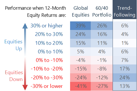
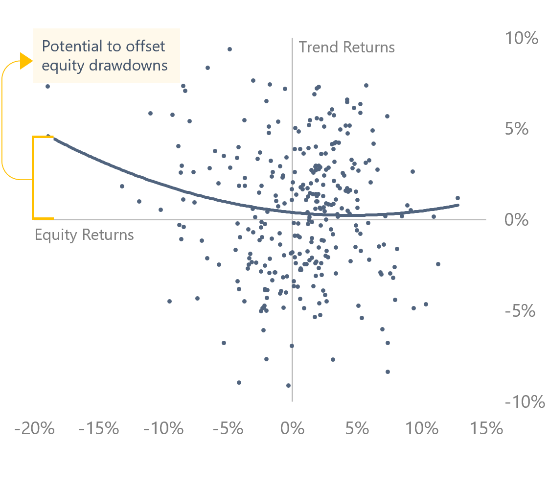
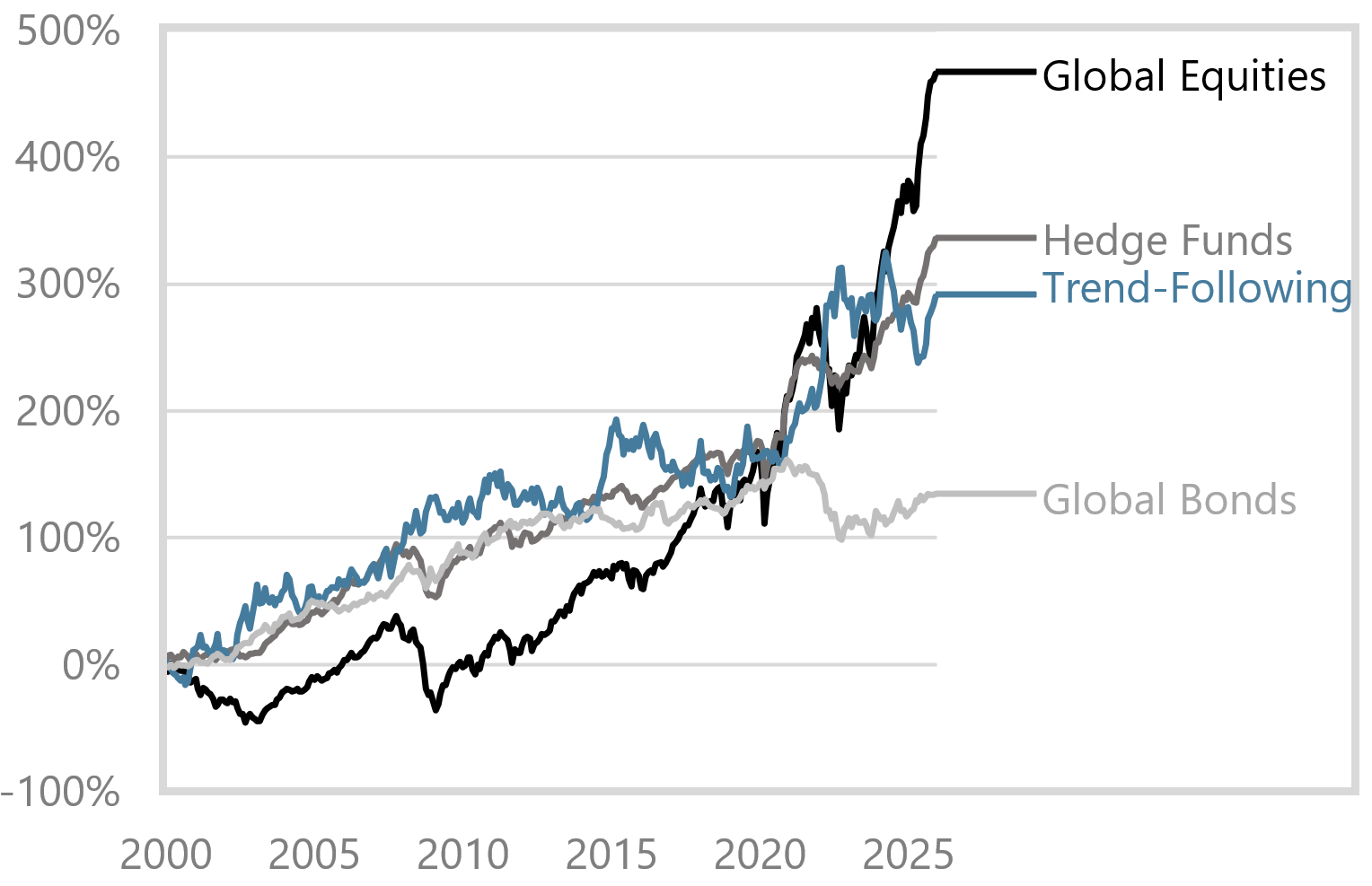
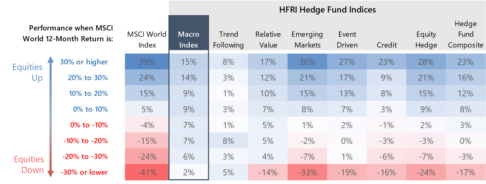
  • Traditional diversification strategies may be less effective in a higher-volatility regime.

INTRODUCTION

A common view is that the pandemic volatility shock was just that: a shock. An exogenous disruption that temporarily pushed markets and the economy off course, but one that is now largely behind us. Inflation has moderated, markets have stabilized, and it is tempting to believe the system is gradually returning to something like the pre-pandemic environment.

Our view is different. We do not believe the pandemic was a one-off disruption to a stable low-volatility regime but was instead the catalyst that exposed the limits of that regime and forced an exit from it. We will argue in this piece that the stability of the post-GFC period was never a natural equilibrium. It depended on a specific macroeconomic backdrop: weak demand, low inflation, disinflationary globalization, and a policy framework able to suppress volatility and inflate asset prices. Those conditions no longer reliably hold.

The result is not simply a more volatile version of the old environment. It is a different regime: one defined by more binding supply constraints, less stable inflation, more active fiscal policy, and a policy framework that is more constrained and less predictable. In that world, volatility is not as easily suppressed. It becomes a structural feature of the system.

Markets have not fully internalized that shift. Asset prices, risk premia, and portfolio construction still reflect assumptions forged in the post-GFC regime, even as the foundation for those assumptions has eroded. The mismatch between how the system is priced and how it now functions is the central risk this piece explores.


HOW AND WHY THE LOW-VOLATILITY REGIME WAS ENGINEERED

To understand why that regime was transitory, it is necessary to understand what created it. The low-volatility environment that followed the Global Financial Crisis was not simply a byproduct of subdued inflation or calmer markets. It emerged from a specific macroeconomic problem, debt deflation, and a specific policy response, asset price reflation.

Debt deflation is dangerous because falling asset prices weaken balance sheets, force deleveraging, reduce credit creation, and push asset prices lower still, creating a self-reinforcing downward spiral. The policy response was therefore clear. If falling asset prices were the problem, rising asset prices were the solution. After the GFC, the Federal Reserve and other major central banks pursued that goal through zero- and negative-rate policy, quantitative easing, forward guidance, and direct asset purchases. These tools did not just stimulate demand. They changed the market pricing of risk: duration risk, term premia, credit risk, equity risk, and volatility itself. Policymakers were not simply trying to restart growth. They were trying to reflate the asset base of the economy.

The Mechanics of Volatility Suppression

Put another way, the tools used to stabilize the post-GFC economy worked in part by suppressing specific market risks. Policymakers could not quickly improve the fundamentals underlying asset prices, but with trillion-dollar balance sheets, they could engineer higher prices by distorting the risks embedded in those prices. Quantitative easing reduced duration risk by removing long-term bonds from the market, inflating the price of duration and, by extension, all long-duration assets from bonds to low-current-cash-flow equities and beyond. Forward guidance compressed uncertainty around the future path of short rates, lowering term premia, and making near-term cash flows less attractive relative to more uncertain, longer-duration ones. Zero-rate policy reduced the time value of money and pushed investors outward along the risk curve. Together, by broadly compressing risk premia, these policies lowered credit spreads, inflated valuations for the longest-duration equities, reinforced the correlation structure that underpinned risk parity and 60/40 portfolios, supported private equity, and made volatility itself appear less risky. But because that market structure depended on inflation remaining low enough for policymakers to keep suppressing risk, it was always more conditional than it appeared.

The Pandemic and the Regime Shift

The pandemic initially triggered an even more aggressive version of the post-GFC policy response. Rates returned to zero, the Fed’s balance sheet nearly doubled from roughly $4 trillion to almost $9 trillion, and fiscal policy was deployed on a scale far beyond the prior cycle, with pandemic relief legislation totaling roughly $5 trillion versus less than $1 trillion for the American Recovery and Reinvestment Act after the GFC.

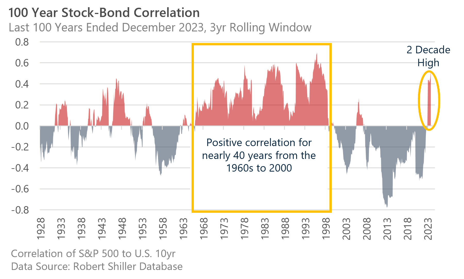
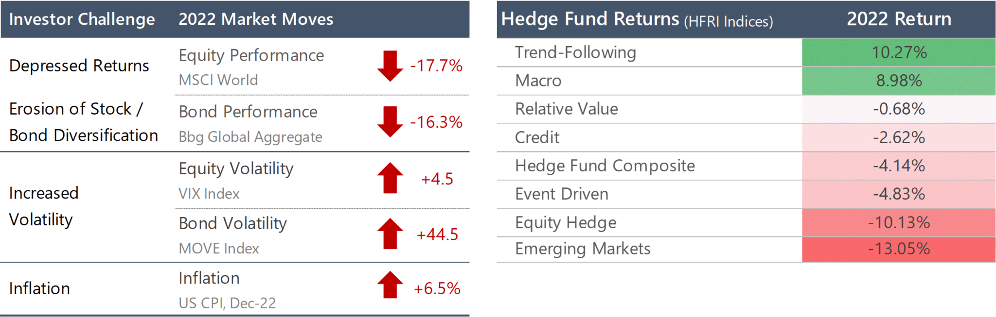
But unlike the post-GFC period, the result was not a prolonged demand shortfall and subdued inflation. It was a rapid recovery in nominal demand, disrupted supply, and the first sustained inflation shock in decades. Once inflation became binding, the Fed was forced to reverse the very policies that had supported the low-volatility regime. Rates rose sharply, balance sheet policy shifted from expansion to runoff, term premia began to reprice, and the negative stock-bond correlation that underpinned the 60/40 portfolio broke down. In 2022, a traditional 60/40 portfolio declined roughly 16–18%, depending on construction, one of its worst performances in modern history. Morgan Stanley estimated 2022 was the worst year for a 60/40 portfolio since 1937 and the fourth-worst in roughly 200 years1.

The issue was not simply that the pandemic was an extreme shock. It was that an extreme shock hit a market structure engineered to treat extreme shocks as unlikely, temporary, and ultimately containable. In that sense, the pandemic did not merely interrupt the low-volatility regime; it exposed the condition on which it had always depended: inflation had to remain low enough for policymakers to keep suppressing market risk.

As markets stabilized, it became tempting to view the pandemic and inflation shock as a one-off disruption to an otherwise durable low-volatility regime. But the low-volatility regime was not a stable equilibrium to which the economy would necessarily naturally return. In this piece, we will argue that low-volatility regime was a conditional construct that depended on macroeconomic and policy conditions that no longer reliably exist. Put simply, when low and stable inflation can no longer be taken for granted, the asset-inflating policies that defined the post-GFC regime can no longer be relied upon either.

The sections that follow explain why the conditions that made volatility suppression possible have eroded.


WHY THE CONDITIONS THAT SUPPRESSED VOLATILITY HAVE BROKEN DOWN

The low-volatility regime was not a naturally occurring phenomenon but was instead the product of a policy framework designed to suppress market risk and inflate asset prices. While policymakers still want to support markets, the question is whether they can still do so without creating larger problems elsewhere. In a higher-inflation environment, easing policy to support markets can backfire by reigniting inflation pressure, pressuring bond yields, and creating new instability. Thus, even as the desire for a policy put may still exist, exercising that put now risks creating the very instability it is meant to prevent.

1. The Economy is More Supply-Constrained Than Demand-Constrained

The post-GFC period was defined by insufficient demand. Volatility was largely tied to growth scares, financial stress, and recurring concerns that the recovery would stall. Those were risks policymakers could offset with easier policy. Lower rates, QE, and forward guidance worked because the economy had spare capacity and inflation was persistently subdued. Liquidity support lifted asset prices and supported demand without immediately creating an inflation problem.

Today, the constraint looks different. The economy appears less demand-deficient and more supply-constrained. Labor force growth has slowed as the population ages, immigration policy has become more volatile, and lower breakeven job growth means the labor market can tighten even with employment gains that would once have looked modest. At the same time, energy, housing, infrastructure, and supply chains have more visible bottlenecks. Even AI, the clearest potential source of faster supply-side growth, is already running into physical constraints. The data-center buildout is colliding with shortages of electricity, grid capacity, transformers, switchgear, batteries, skilled labor, and construction capacity. Bloomberg recently reported that almost half of U.S. data centers planned for this year are expected to be delayed or canceled because of shortages in electrical equipment, and this was before any further supply disruptions that may come from the Iran conflict2.

That changes the policy tradeoff. In a demand-constrained economy, liquidity is stabilizing: it lifts asset prices, supports demand, and does not immediately threaten inflation. In a supply-constrained economy, the same liquidity is more dangerous. It pushes demand into bottlenecks, raises prices, and forces policymakers to choose between supporting markets and preserving inflation credibility.

2. Inflation Can No Longer Be Treated as Dormant

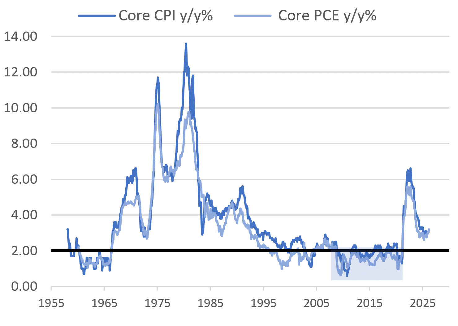
Inflation can no longer be assumed to be safely contained. In the post-GFC period, inflation was persistently too low: core PCE inflation averaged below the Fed’s 2% target for most of the decade following the crisis, even as unemployment fell below 4% by 2018. Structural forces like demographics, globalization, technology, and anchored expectations were keeping inflation subdued and the persistence of those factors gave the Fed and other major central banks room to keep policy easy, use forward guidance and balance-sheet expansion. Those policies suppressed volatility and supported asset prices with few immediate inflationary consequences.

The pandemic broke that assumption. It showed that when policy supports demand into a constrained supply environment, inflation can re-emerge quickly and forcefully. More importantly, it showed that inflation is not as inert as previously believed. It is not simply a lagging outcome that can be managed over time, but a variable that can move rapidly when conditions change.

Source: Graham Capital Management

The pandemic may also have changed pricing behavior itself. After a long period in which firms were reluctant to raise prices and consumers were conditioned to expect price stability, the inflation shock made price increases more visible, more frequent, and more accepted as a response to cost pressure. That does not mean inflation will remain high indefinitely, but it does suggest pricing behavior may be more dynamic than it was during the post-GFC period. In that environment, inflation can become less inert and more responsive to shocks.

Source: BEA, FRB/Haver

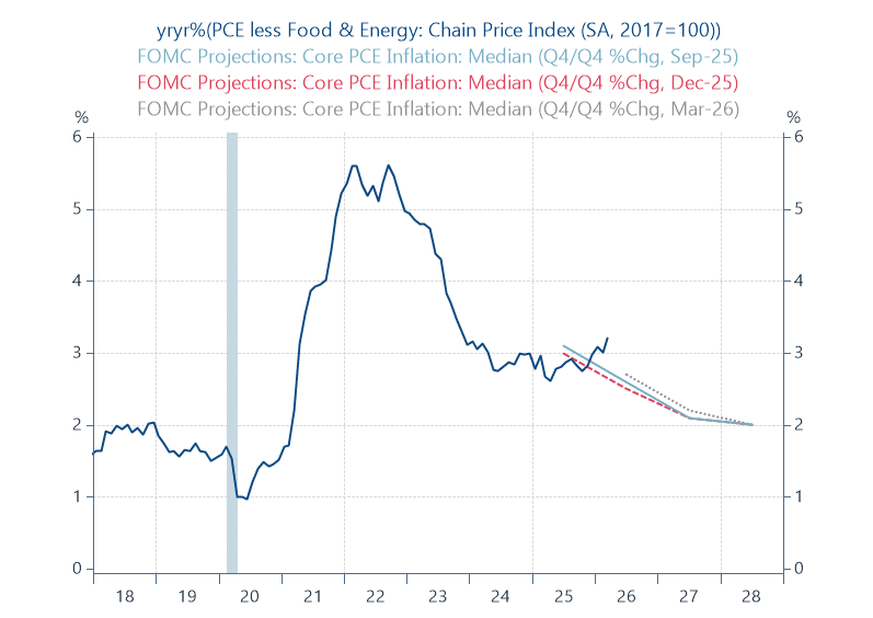
This fundamentally changes the policy framework. There is an obvious incentive, from both policymakers and markets, to return to the pre-pandemic model. But as the economy has suffered from persistent supply constraints, inflation has also proven more persistent than hoped. At the same time, asset markets remain acutely sensitive to sharp moves higher in government bond yields, and policymakers can no longer assume that weakness in growth or markets will automatically create room to ease. The Fed is now operating with a constraint that was largely absent in the post-GFC period: the risk that policy support itself reignites inflation.

3. Globalization Is No Longer a Reliable Disinflationary Force

The pandemic also exposed the limits of globalization as a volatility suppressor. In the post-GFC period, global supply chains helped keep goods prices low and allowed shocks to be absorbed across a broad, flexible production network. That was part of what made inflation look structurally contained. Even when demand improved, firms could rely on global labor, cheaper imported goods, and just-in-time production to limit cost pressures.

That dynamic started to break during the pandemic. Supply chains that had been optimized for efficiency proved more fragile than expected, and the initial shortages made clear that low-cost production was not the same thing as resilient production. Since then, the shift has accelerated. Tariffs, industrial policy, export controls, reshoring, and the deterioration of diplomatic alliances have all pushed the system further away from maximum efficiency and toward redundancy, security, and political control.

That shift may be justified from a national security or resilience perspective, but it is not disinflationary. A world with more fragmented supply chains, more trade barriers, and more politically directed production is a world with less elastic supply and higher costs. Shocks that might once have been absorbed through global production networks are now more likely to persist, feed into prices, and complicate policy.

This is not just a U.S. story. The broader environment that helped suppress inflation has also shifted. Europe has moved away from austerity toward more active fiscal policy, reducing a key source of demand restraint. Japan, long a source of persistent disinflation, is now experiencing sustained inflation and shifting away from ultra-loose policy. The post-Brexit U.K. has become an example of how reduced trade openness and a less elastic labor supply can leave an economy more vulnerable to persistent inflation. More broadly, geopolitical fragmentation, trade barriers, and shifting alliances are making the system less efficient and less disinflationary.

4. Fiscal Policy Has Become a Source of Volatility

Another important shift is the role of fiscal policy. In the post-GFC period, fiscal policy was generally more constrained, particularly in the U.S. After the initial crisis response, many advanced economies moved toward austerity or at least fiscal restraint, in part because markets had become more intolerant of high and rising sovereign debt burdens. Europe was the clearest example: countries with the weakest fiscal positions experienced the sharpest sovereign bond-market volatility, with spreads and yields in countries like Italy and Greece rising sharply, while countries with stronger balance sheets were less exposed. That distinction matters because it shows that fiscal sustainability itself can become a source of market instability. In the post-GFC period, that pressure pushed policy toward restraint, reinforcing the demand shortfall and reducing pressure on inflation.

Fiscal restraint also supported the low-volatility goals of monetary policy more directly. Lower deficits meant reduced Treasury issuance, which helped keep term premia and duration risk contained. Combined with QE, this created a powerful dynamic: central banks were removing duration from the market at the same time that governments were not meaningfully increasing its supply. The result was a structurally lower level of long-term yields, compressed risk premia, and reduced rate volatility. Fiscal and monetary policy were aligned in actively suppressing market risk.

Source: Graham Capital Management

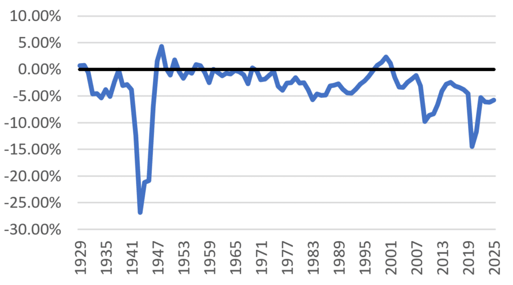
That alignment has broken down. Fiscal policy has become larger, more persistent, and less tied to the cyclical stabilization role it played in the post-GFC framework. The pandemic marked a clear turning point, with deficits expanding dramatically and fiscal support continuing well into the recovery. Since then, fiscal policy has remained active through industrial policy, defense spending, energy transition investments, and supply-chain resilience programs, including legislation such as the CHIPS Act, the Inflation Reduction Act, and increased defense commitments.
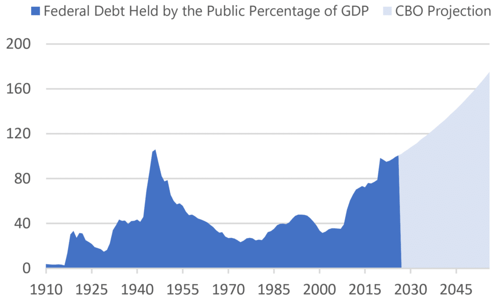
Source: Graham Capital Management

The issue is not just the scale of fiscal policy, but also its composition. More recent fiscal support has often been directed toward defense, transfers, subsidies, industrial policy, and energy security rather than higher-multiplier public investment. To the extent that this spending sustains demand without generating a commensurate increase in near-term supply, it can be more inflationary and less growth-enhancing. That makes fiscal policy a less reliable stabilizer and a more direct source of volatility.

Fiscal policy now works in the opposite direction of the post-GFC regime. Instead of reinforcing demand weakness, it can amplify demand at a time when supply is already constrained. Larger deficits also mean increased Treasury issuance, which can put upward pressure on long-end yields even as the Fed attempts to manage financial conditions. In that environment, efforts to support markets, whether through easier monetary policy, fiscal stimulus, or public pressure to keep financial conditions loose, can be offset or even overwhelmed by the bond market’s reaction to fiscal expansion.
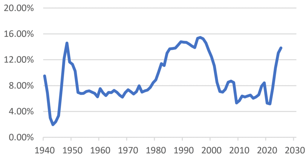
Source: Graham Capital Management

5. Economic Signals Are Harder to Interpret

While all these changes have occurred, the economy itself has become harder to read. In the post-GFC period, growth was weak, but the underlying structure of the economy was relatively stable. Estimates of labor supply, potential growth, and slack were imperfect, but they were not moving targets. Policymakers could make decisions with a reasonable degree of confidence about the economy they were trying to manage.

That is less true today. Key inputs into monetary policy are more uncertain and more dynamic. Productivity may be shifting because of AI, but the timing and magnitude are unclear. Labor supply is being reshaped by aging and reduced immigration, making it harder to know how tight the labor market really is. Recent Fed staff research3 has argued that slower labor-force growth may have reduced breakeven employment growth to near zero, meaning payroll gains that once would have signaled expansion may now be consistent with a tightening labor market. At the same time, declining resources at government statistical agencies4 have introduced additional measurement error, making the data themselves less reliable just as the economy has become harder to interpret. The relationship between growth, wages, and inflation has also become less stable.

That instability makes the key inputs into policy harder to estimate in real time: actual growth, potential growth, and the neutral policy rate. Policymakers are forced to infer the state of the economy from less reliable data that can support multiple, often conflicting interpretations. Strong growth could reflect improved supply or overheating demand. Slower hiring could signal weakness or simply a lower labor force growth rate. Sticky inflation could reflect demand, supply constraints, or both.

This uncertainty matters because policy is set based on those inferences. In a recent speech, Fed Governor Christopher Waller raised the possibility that the Fed may have misread weak payroll gains as labor-market deterioration when they may have instead reflected sharp declines in labor availability5. If policymakers had understood that distinction in real time, it is not clear they would have eased as they did. That is exactly the kind of observability problem that can turn into policy error. Because those mistakes are only revealed with a lag, the eventual adjustment may need to be larger and more abrupt. In that sense, the challenge is no longer just uncertainty but also unobservability, and that makes for a less stable backdrop for both policy and markets.

Taken together, these changes mean the policy framework that suppressed volatility after the GFC has fewer degrees of freedom. Weak demand, low inflation, elastic global supply, fiscal restraint, and stable financial conditions gave policymakers room to ease aggressively without immediately creating offsetting risks. That room has narrowed. Policy support can still stabilize markets, but it can also push demand into bottlenecks, reignite inflation pressure, raise long-end yields, weaken credibility, or force a larger adjustment later. The policy put has not disappeared, but it has become more costly to exercise and therefore less reliable.

MARKETS ARE STILL PRICED FOR THE OLD REGIME

If the post-GFC regime was defined by suppressed volatility, compressed risk premia, and a policy framework that reliably supported asset prices, then the implications of its reversal are not subtle. Markets are still priced as if much of that regime remains intact, even as the conditions that supported it have weakened.

The starting point is the price of risk. Risk premia are often discussed as abstract valuation concepts, but in practice they determine how much leverage the system can support, how expensive hedging is, how tight credit spreads can remain, how high equity multiples can go, and how low long-end yields can stay. When risk premia are compressed, the same cash flows support higher asset prices. When risk premia rise, those prices fall, even if the cash flows themselves have not changed.

Term premia are the clearest example. By 2019, term premia had fallen to roughly -150 basis points, a level difficult to justify under any normal understanding of risk pricing. Investors were not merely receiving too little compensation for duration risk. They were effectively paying to hold it. As inflation returned and the Fed tightened policy, term premia moved toward roughly +50 basis points. That repricing was part of the broader rate shock that helped break the traditional 60/40 portfolio in 2022.

Markets may be treating that repricing as finished when it was only the first adjustment. Even after the move from deeply negative levels, term premia remain well below longer-run averages and far below levels reached when inflation risk was priced more aggressively. What markets are treating as a completed adjustment may still reflect a significant degree of complacency. If the macro environment has changed, a further move higher in term premia would raise long-end yields even without a change in expected short rates, tighten financial conditions, pressure equity multiples, and force investors to reprice long-duration assets across the system.
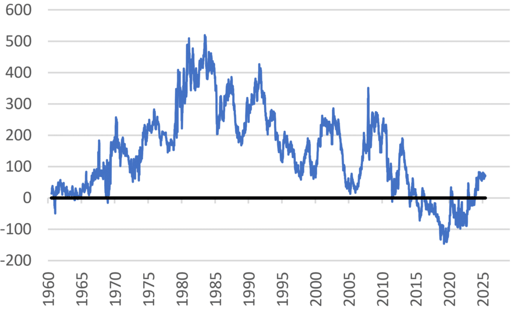
Source: New York Fed Adrian/Crump/Moench (ACM) model estimates of Treasury term premia.

That is why term premia matter. They are not an abstract bond-market concept. They are one of the prices that determine the valuation of every long-duration asset in the system. When term premia are low, long-duration assets look safer, equity multiples can rise, bonds can hedge equities, credit spreads can remain tight, and leverage can build. When term premia rise, all of that changes.

This is the broader mistake markets may be making. Many of the features investors came to treat as constants were actually regime-specific variables. Negative stock-bond correlation was not a permanent law of portfolio construction; it depended on low and stable inflation. Higher valuations for long-duration equities were not a permanent feature of superior business models; they depended on low discount rates and low required returns. Tight credit spreads were not simply evidence of stronger corporate fundamentals; they were partly the result of investors being pushed outward along the risk curve. Private equity valuations were not insulated from the public-market regime; they were one of its clearest expressions.

That is the key point. The post-GFC regime did not just raise asset prices. It changed the way investors understood risk. It made duration look safer, leverage look more sustainable, illiquidity look less costly, and volatility look more suppressible. Those assumptions worked because inflation was low, policy was predictable, and central banks could respond to weakness by easing. If those conditions no longer hold, then the assumptions built on top of them no longer hold either.


THIS IS HOW THE OLD ASSUMPTIONS BREAK

If the assumptions of the post-GFC regime are still embedded in prices, then the consequences are not theoretical. Many assets and portfolios still reflect assumptions about inflation, policy, and risk that no longer reliably hold. As those assumptions are tested, the adjustment will show up in how risk is priced across markets. Some of that adjustment has already happened. The mistake is assuming it is finished.

1. High Multiples Do Not Need Weak Earnings to Fall

High equity multiples are one place where the mismatch is most visible. U.S. equities remain historically expensive, with the S&P 500 trading around 22x forward earnings, above its 30-year average of roughly 17x6, while the CAPE ratio is near 38x, more than double its long-run average of roughly 17x7. The issue is not simply that valuations are high. It is that they are high for reasons that may no longer be valid.

The multiple expansion of the post-GFC period was not driven by earnings alone. It was driven by falling discount rates, compressed term premia, suppressed volatility, and the expectation that policymakers would cushion drawdowns. Those conditions made future cash flows look more valuable and reduced the compensation investors demanded for uncertainty.

A rerating would still likely require a catalyst, so this is not a near-term market call. But the vulnerability is already embedded in the starting valuation. If the forward multiple merely returned to its long-run average, that would imply roughly 20% downside before any change in earnings. If multiples moved to levels more consistent with higher inflation or higher-volatility environments, the adjustment would be larger. The point is not the precise downside estimate. The point is that equities do not need an earnings collapse to fall. The same stream of cash flows can support a lower price simply because investors demand more compensation to hold it.

A valuation reset does not require a recession or a replay of the 1970s. It only requires investors to stop paying post-GFC multiples for cash flows in a world that no longer supports post-GFC assumptions.

2. Smooth Marks Are Not the Same as Low Risk

The same dynamic is visible in private credit and other illiquid assets. Their appeal has been the ability to generate stable income with limited mark-to-market volatility. But that stability is, in part, a function of how the assets are priced.

Less frequent pricing can make volatility look lower without making the underlying risk lower. In an environment of low rates, abundant liquidity, and easy refinancing conditions, that distinction mattered less. Defaults were low, capital was readily available, and time worked in the investor’s favor.

That environment is less reliable now. Higher rates, tighter financial conditions, and greater macro volatility make refinancing more uncertain and increase the importance of liquidity. In that world, the absence of daily marks does not eliminate volatility. It delays its recognition.

The risk is that illiquidity has been treated as a source of return rather than a source of risk. In a regime where the price of risk rises, illiquidity should require more compensation, not less.

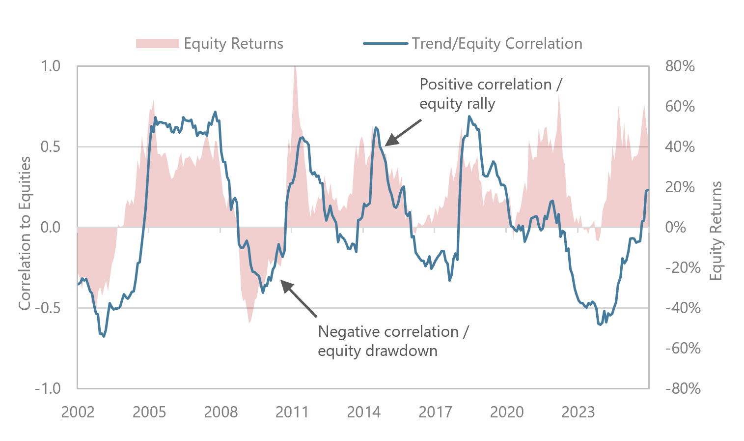
3. Diversification Still Depends on the Inflation Regime

One of the most important assumptions carried forward from the post-GFC period was that bonds would reliably diversify equity risk. That assumption mattered most for risk parity and other volatility-targeted strategies, which depended not only on bonds rallying when equities fell, but on the stock-bond correlation remaining stable enough to support leverage. The traditional 60/40 portfolio benefited from the same structure, but risk parity, which gained traction in the post-GFC period, was more directly exposed to it. When inflation shocks pushed stocks and bonds down together in 2022, the problem was not simply that bonds failed to hedge equities. It was that a core input into the portfolio construction process had changed.
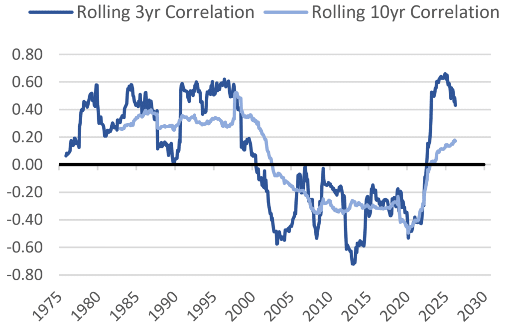
Source: Graham Capital Management

That relationship is not a law of nature. It depends on the inflation regime. In a low and stable inflation environment, shocks tend to be growth shocks. Policy can ease in response, bond yields fall, and bonds hedge equities. That dynamic underpinned the performance of balanced portfolios for much of the post-GFC period.

In a higher and less stable inflation environment, that relationship becomes less reliable. Shocks are more likely to be inflation shocks, or a combination of inflation and growth. In that case, policy cannot respond as easily, bond yields can rise alongside equity volatility, and the hedge weakens or disappears.

That is what happened in 2022, when both stocks and bonds declined sharply. The point is not that diversification no longer works. It is that diversification is conditional. Portfolios that appear diversified across asset classes may still be concentrated in a single underlying assumption: that inflation remains low and that policy can respond to weakness without constraint.

4. Regime Change Looks Like a Series of One-Off Shocks

If the repricing of risk is not complete, it is unlikely to happen in a smooth or linear way. Regime changes rarely do. They tend to unfold through events that initially appear unrelated.

That is what this period has felt like. Even after the pandemic volatility seemed to have passed and markets tried to return to the old normal, the shocks continued. August 2024 brought a sharp global selloff tied to recession fears, crowded positioning, and the yen carry-trade unwind. April 2025 brought tariff-driven volatility and a sharp move higher in Treasury yields. March 2026 brought another broad selloff, this time tied to tariffs, AI-capex concerns, private-credit liquidity worries, and geopolitical risk. Each episode had its own catalyst. But the frequency matters. When large disruptions keep arriving every few months, the better question is whether they are really isolated shocks at all.

Each episode can still be explained in isolation. That is what makes the transition difficult to recognize in real time. The impulse is to interpret each shock through the old framework: volatility will fade, policy will respond, markets will stabilize. That was often the right reflex in the post-GFC regime.

In a different regime, that reflex can be misleading. What looks like a series of temporary disruptions may instead be the process through which risk is repriced. The adjustment does not need a single defining event. It can emerge through repeated shocks that stop looking isolated only in hindsight. Regime changes are not recognized as regimes until repeated “one-off” shocks stop looking isolated.


The economy is increasingly leveraged to asset prices not falling, while the tools used to support those prices are increasingly constrained by inflation, deficits, and the bond market. That is the tension running through this regime shift. The policy put has not disappeared, but it is less reliable, less powerful, and more costly to exercise. The excesses of the post-GFC regime have not been fully unwound. They have been carried forward into a new environment that is less capable of sustaining them. Markets are still priced for stability in a system that is becoming structurally less stable.


CONCLUSION

After a rupture, continuity is the most seductive illusion: the belief that the old order is still there, temporarily obscured but fundamentally intact. For more than a decade, that instinct was not only understandable; it was profitable. It was also enforced by central banks, which penalized investors who positioned against it. The post-GFC regime trained investors to think in a certain way: buy duration, buy dips, own the market, accept illiquidity, add leverage, trust that bonds would hedge equities, and assume that policymakers would eventually step in. Those were not irrational choices. They were the correct choices for a world of low inflation, weak demand, compressed risk premia, and policy-suppressed volatility. But they were regime-specific choices, not universal truths — and habits formed in one regime can become liabilities in the next.

If the regime has changed, then the question is not whether 60/40 is “dead,” whether equities are “too expensive,” or whether bonds “work” again. Those questions are too narrow. The better question is whether investors are still using a playbook built for a world that no longer exists. A 60/40 portfolio may still look diversified, but if both sides depend on low inflation and low term premia, it is less diversified than it appears. Private assets may still look smooth, but smoothing is not the same thing as safety. Long-duration equities may still have great businesses behind them, but great businesses can still be bad assets at the wrong discount rate.

The trade, broadly speaking, is not to assume disaster. It is to stop assuming rescue. It is to stop treating volatility as a policy mistake that will always be corrected and start treating it as a feature of the new environment. That means caring more about valuation, cash flow timing, liquidity, inflation sensitivity, and whether the hedge is really a hedge. It means recognizing that many portfolios that look diversified by asset class may actually be concentrated in one underlying exposure: the assumption that risk will remain underpriced.

Regime changes are rarely recognized cleanly in real time. They often arrive as a series of events that look separate at first: an inflation shock, a bond bear market, a 60/40 drawdown, a yield spike, a growth scare. Each can be explained away on its own. But taken together, they may be evidence of something larger: not repeated disruptions to the old regime, but the emergence of a new one.

The low-volatility regime made leverage look prudent, illiquidity look safe, long-duration cash flows look inherently superior, and diversification look almost automatic. A higher-volatility regime is likely to reverse that illusion. It does not eliminate opportunity, but it changes where opportunity lies. It favors assets whose returns come from current cash flows and reasonable starting valuations, not from falling discount rates, multiple expansion, or policy rescue. The opportunities will still be there, but not for portfolios built on yesterday’s assumptions. Those assumptions will be obstacles, not guides.

IMPORTANT DISCLOSURE

REFERENCES​

1 Morgan Stanley Investment Management. ‘BIG PICTURE: Return of the 60/40.’ Morgan Stanley Investment Management, April 2024, https://www.morganstanley.com/im/publication/insights/articles/article_bigpicturereturnofthe6040_ltr.pdf. Accessed 5/13/2026.

2 Bloomberg. ‘US Data Center Boom Relies on Hard-to-Find Electrical Equipment.’ Bloomberg, April 1, 2026, https://www.bloomberg.com/news/newsletters/2026-04-01/us-data-center-boom-relies-on-hard-to-find-electrical-equipment. Accessed 5/13/2026.

3 Board of Governors of the Federal Reserve System. ‘Labor Force Growth, Breakeven Employment, and Potential GDP Growth.’ Federal Reserve, April 2, 2026, https://www.federalreserve.gov/econres/notes/feds-notes/labor-force-growth-breakeven-employment-and-potential-gdp-growth-20260402.html. Accessed 5/13/2026.

4 U.S. Bureau of Labor Statistics. ‘Notice of CPI Collection Reductions.’ Bureau of Labor Statistics, 2025, https://www.bls.gov/cpi/notices/2025/collection-reduction.htm. Accessed 5/13/2026.

5 Board of Governors of the Federal Reserve System. ‘Labor Market Data: Signal or Noise?’ Federal Reserve, February 23, 2026, https://www.federalreserve.gov/newsevents/speech/waller20260223a.htm. Accessed 5/13/2026.

6 J.P. Morgan Asset Management. ‘Guide to the Markets.’ J.P. Morgan Asset Management, https://am.jpmorgan.com/us/en/asset-management/adv/insights/market-insights/guide-to-the-markets/. Accessed 5/13/2026.

7 Shiller, Robert. ‘Online Data Robert Shiller.’ Yale University Department of Economics, http://www.econ.yale.edu/~shiller/data.htm. Accessed 5/13/2026.

LEGAL DISCLAIMER

This presentation includes statements that may constitute forward-looking statements. These statements may be identified by words such as “expects,” “looks forward to,” “anticipates,” “intends,” “plans,” “believes,” “seeks,” “estimates,” “will,” “project” or words of similar meaning. In addition, our representatives may from time to time make oral forward-looking statements. Such statements are based on the current expectations and certain assumptions of Graham’s management, and are, therefore, subject to certain risks and uncertainties. A variety of factors, many of which are beyond Graham’s control, affect the operations, performance, business strategy and results of the accounts that it manages and could cause the actual results, performance or achievements of such accounts to be materially different from any future results, performance or achievements that may be expressed or implied by such forward-looking statements or anticipated on the basis of historical trends.
This document is not a private offering memorandum and does not constitute an offer to sell, nor is it a solicitation of an offer to buy, any security. The views expressed herein are exclusively those of the authors and do not necessarily represent the views of Graham Capital Management. The information contained herein is not intended to provide accounting, legal, or tax advice and should not be relied on for investment decision making.

Trend-Following Primer

Trend-following is among the most established and longest-standing investment strategies, with an estimated $350 billion1 in assets under management globally. Rooted in the premise that markets tend to exhibit persistent directional movements over time, trend-following seeks to capture these trends across a broad set of asset classes using disciplined, rules-based processes. By taking both long and short positions in liquid global markets, the strategy has historically demonstrated low correlation to traditional assets and the ability to perform across a range of market environments. As investors increasingly seek diversification and resilience in portfolios, trend-following has become a strategic allocation within many institutional investment frameworks. This primer outlines the key characteristics of trend-following and explores how the strategy can impact a broader investment portfolio when implemented as a long-term, strategic allocation.

Key Takeaways

  • Trend-following has historically exhibited low correlation to traditional assets and can provide diversification across market environments.
  • By taking both long and short positions, trend-following can perform during sustained market moves, including periods of market stress.
  • Incorporating trend-following may improve portfolio outcomes by enhancing returns while reducing volatility, drawdowns, and equity sensitivity over time.

WHAT IS TREND-FOLLOWING?​

Trend-following strategies use a systematic process, whereby algorithmic models seek to identify price trends in markets, with the expectation that upward trending markets may continue to rally and downward trending markets may continue to decline. These strategies take long positions in positively trending markets and short positions in negatively trending markets, using indicators based on price and volatility of the underlying assets to identify trends of various lengths. Trend followers seek to run diverse portfolios, typically trading liquid, centrally-cleared futures and currency markets, with the number of markets potentially ranging from tens to hundreds. These strategies often target consistent volatility within a predetermined range and try to preserve upside potential and limit downside risk by running with winners and cutting losing positions.

Theoretical Foundation: Why Do Markets Trend?
Trend-following performance depends on the existence of trends, or sustained directional moves in markets. Trends may exist both in times of market duress or during relatively stable market environments. A substantial body of academic research supports the existence of trends and offers several explanations for why they persist across asset classes:

  • Behavioral Bias and Herding Investors extrapolate recent price movements into the future and “follow the crowd,” reinforcing trends (Barberis, Shleifer, and Vishny, 1998; Bikhchandani, Hirshleifer, and Welch, 1992).
  • Anchoring and Underreaction Investors adjust too slowly to new information, leading prices to trend as markets gradually incorporate news (Tversky and Kahneman, 1974; Hong and Stein, 1999).
  • Disposition Effect Investors sell winners too early and hold onto losers (Frazzini, 2006).
  • Risk Management Risk constraints can force investors to buy or sell assets as volatility or risk limits change, amplifying existing price moves (Danielsson, Shin, and Zigrand, 2012).
  • Macroeconomic Regimes Shifts in monetary and fiscal policy can drive sustained trends across asset classes as markets reprice growth and inflation expectations (Ang and Bekaert, 2007).
  • Time-Varying Risk Premia Changes in the compensation investors require to hold risky assets can lead to prolonged price movements across asset classes (Moskowitz, Ooi, and Pedersen, 2012).

Together, these behavioral and structural forces help explain why trends can emerge and persist, forming the foundation for trend-following strategies.


TREND IDENTIFICATION

Trend-following strategies identify trends by systematically analyzing historical market prices. Algorithms evaluate price movements over lookback periods ranging from intraday to several months to determine whether a market is exhibiting sustained upward or downward momentum. When prices rise consistently, models may take long positions; when prices decline, they may take short positions.

Models also incorporate price volatility and other risk measures to determine position sizing and overall portfolio exposure. More volatile markets typically receive smaller allocations, while less volatile markets may receive larger/f positions to maintain balanced risk across a diversified set of assets such as equities, interest rates, currencies, and commodities.

Signal Generation

Moving average and breakout models are two prominent strategies used by most trend-followers for initial signal generation. While these models may be parameterized differently, the raw signals generated are often highly correlated over time because of their common dependence on past prices.

Breakout models compare the current price with a threshold to signal long, short, or no position. The threshold is determined by either a “price breakout” (past maximum or minimum price) or “channel breakout” (past price at a given lookback and trading range.)

Source: Graham Capital Management

Moving Average Models use moving averages of past prices to generate a trading signal. The difference between two moving averages, a “fast” and a “slow” one, determines a long or a short position. A crossover between the two will signal a trend reversal.

Source: Graham Capital Management

While these approaches differ in construction, they share a common objective: detecting persistent directional movement in prices. A key factor influencing how these models behave is the speed at which they respond to new information, which is largely determined by parameter choices such as lookback windows and signal thresholds.


THE SPEED OF TREND-FOLLOWING

A key dimension of trend-following strategies is speed, which refers to how quickly a model responds to emerging price movements. Speed is primarily determined by model parameters such as the length of moving averages and breakout lookback windows. Models that use shorter lookback periods are typically considered faster (short-term trend-following), as they respond more quickly to recent price changes and may identify new trends earlier. Slower models, which rely on longer lookback horizons (long-term trend-following), tend to react more gradually but may be less sensitive to short-term market noise. As a result, faster models can adapt more quickly to changing market conditions but may experience more frequent position changes and potential “whipsaws,” while slower models may capture longer, more persistent trends with fewer trades.

Evidence across time suggests that model speed can influence performance depending on market conditions. As shown in the heatmap below, which compares the performance of trend models across different time horizons, intermediate- to longer-term models have, on average, fared better than shorter-term models. When longer-term signals performed well, faster models often produced similar gains, though the reverse was less frequently the case.

However, faster models can be particularly valuable during periods of sudden market dislocation, when trends emerge quickly. For example, during episodes of sharp market stress such as the early stages of the COVID-19 crisis in 2020, faster signals were able to react more quickly. As a result, incorporating shorter-term models can help strategies respond more quickly during abrupt market events, complementing slower models that capture more persistent trends.

As a result, when selecting the speed of trend signals, many managers use a blend of signal speeds to balance responsiveness, cost efficiency, and robustness across different market environments.


MARKETS TRADED

Trend-following typically trades a diversified set of liquid global markets, most commonly through exchange-traded futures and forwards. These instruments provide efficient access to major asset classes, including equities, fixed income, currencies, and commodities, and allow trend-followers to take both long and short positions. Because futures markets are liquid, centrally cleared, and relatively low cost to trade, portfolios often include dozens – or up to hundreds – of markets across global regions. Diversification across markets is a core feature of trend-following, as trends can emerge in different asset classes at different times.

Considerations in Market Selection
Considerations for including markets in a trend-following portfolio include the potential alpha opportunity, correlation with existing holdings, liquidity, price history, transaction costs, and operational complexity. While some alternative or niche markets may exhibit strong trends, they can be more difficult to trade at scale due to lower liquidity, wider spreads or operational complexity. As a result, managers must weigh the incremental diversification and return potential against implementation challenges and costs. Legal and regulatory constraints also play an important role, as certain instruments or jurisdictions may impose restrictions on derivatives usage, margin requirements, reporting, or fund structures, particularly in vehicles such as UCITS or ‘40 Act funds. These considerations can influence which markets are included and how exposures are implemented within a given strategy.


PORTFOLIO CONSTRUCTION

Beyond choices related to signal generation, model speed, and the markets traded, portfolio construction plays a critical role in determining how signals are combined across the portfolio, how risk is allocated across markets, and how exposures are scaled while maintaining disciplined risk management.

Combining and Weighting Signals
Managers must determine how to combine and weight signals from multiple models and time horizons into a composite forecast that reflects the overall strength and direction of trends in each market. Considerations include historical signal quality, volatility and correlation to other signals, among other factors. Combining signals helps reduce reliance on any single model specification and can improve the consistency of trend detection.

Volatility Targeting and Leverage
Many trend-following strategies employ volatility targeting to maintain a relatively stable level of portfolio risk. Position sizes are scaled based on the volatility of each market, so more volatile assets receive smaller allocations and less volatile markets receive larger positions. Because futures markets require relatively little margin to gain exposure, leverage is often used to scale the overall portfolio to a target level of risk.

Volatility targeting can be implemented in different ways. Managers may differ in how volatility is measured and targeted across time horizons to balance responsiveness and stability, with the choice reflecting a preference for either stability or adaptability to changing market environments while maintaining overall portfolio risk within a desired range. Some managers use constant volatility targeting, adjusting exposures to maintain a fixed portfolio volatility level over both short and long time horizons. Others use dynamic volatility targeting, allowing the volatility to vary with market conditions or changes in risk estimates.

Risk Management
Managers typically apply risk controls such as position limits for individual markets, caps on sector or asset class exposure, and portfolio-level constraints. These measures help prevent excessive concentration in correlated markets and aim to ensure that portfolio risk remains diversified and controlled across changing market environments.


PERFORMANCE CHARACTERISTICS OF TREND-FOLLOWING

Trend-following has historically shown low correlation to traditional assets and the ability to perform in both rising and falling markets. Over time, it has delivered positive long-term returns with convex performance during sustained trends, including periods of market stress.

Please note: Equities and bonds are represented by the MSCI World Index and the Bloomberg Global Aggregate Index, respectively, unless otherwise noted. Please refer to the important disclosures at the end of this presentation.

Non-correlated returns

Over the long-term, trend-following has had low or even negative correlation to other investments. Trend following strategies also tend to exhibit negative downside correlation to equity markets, providing the potential to perform well during periods of sustained stress in global equity markets. At any point in time, however, correlations may be positive or negative, including during crisis conditions. Therefore, trend following strategies should not be treated exclusively as a portfolio hedge; rather, they may be viewed as additional sources of uncorrelated returns over intermediate to longer-term time periods.

Data Source: Societe Generale, eVestment

No Structural Long or Short Bias

No structural long or short bias means that correlations may be positive or negative over different time horizons. On average, trend-following has no correlation to the markets that it trades and typically has positive correlation when markets move higher and negative correlation when markets decline.

Data Source: Societe Generale, eVestment; Chart by Graham Capital Management

Because trend-following has no structural long or short bias, it can generate returns in both rising and falling markets and potentially perform well across different phases of the market cycle, as illustrated below.

Data Source: Societe Generale, eVestment; Chart by Graham Capital Management

Positive Convexity

Trend-following exhibits positive convexity, or a non-linear pay-off to its underlying market universe. This is a highly valued characteristic for investors seeking portfolio diversification. As shown below, trend-following performs well during large directional moves (up or down), including equity stress periods. In these environments, the strategy can capture extended trends and generate outsized gains, while typically experiencing more limited losses during smaller or less persistent market moves.

Convexity of Trend-Following to Equities

Since SG Trend Index Inception (Monthly Returns, Jan-00 to Dec-25)

Data Source: Societe Generale, eVestment; Chart by Graham Capital Management

Potential to Offset Equity Drawdowns

Trend-following has historically performed well, on average, during equity sell-offs, but positive performance during equity downturns is not guaranteed. For example, while trend-following was a good hedge during longer-term market declines such as the burst of the technology bubble and the Global Financial Crisis, it did not provide protection during the shorter-term equity sell-off in Q4 2018. Importantly, sharp reversals and short-term declines can be challenging for trend-following.

Data Source: Societe Generale, eVestment; Chart by Graham Capital Management

Market Inflection Points

Trend-following can face challenges around market inflection points, when the direction of prices changes abruptly after an extended trend. Because models rely on past price behavior to confirm trends, they often enter after a move has begun and exit after a reversal is evident. As a result, strategies may experience losses during short, sharp market drawdowns, when prices rapidly shift direction, as positions are unwound before new trends are established. As illustrated in the figures below, performance tends to improve during more sustained equity drawdowns, while shorter, abrupt episodes can be more challenging, reflecting the design of trend systems to capture persistent moves rather than predict turning points.

Data Source: Societe Generale, Bloomberg; Chart by Graham Capital Management
Trend-Following Returns and Equity Drawdown Length
Based on Daily Returns Jan-00 to Dec-25; MSCI World Drawdowns <-10%
Data Source: Societe Generale, Bloomberg; Chart by Graham Capital Management

Trend-Following Across Volatility Regimes

It is well-documented that trend-following generally performs well during crisis periods for equities. Since market volatility tends to spike during equity crisis periods, many investors are tempted to characterize trend-following as a long volatility strategy. Contrary to such an interpretation, trend-following can perform well in both high and low volatility environments. It is the existence of sustained market trends rather than high volatility that preconditions good trend-following performance. Using the VIX Index as a measure of market volatility, trend-following performance can be observed to perform well in both high and low volatility regimes, as shown below.

Data Source: Societe Generale, eVestment; Chart by Graham Capital Management

Hypothetical Example of Low Volatility Asset
Consider a hypothetical asset that goes down 1% every day. Any reasonable implementation of trend-following would short this asset and thereby make a certain gain on an asset that itself has no volatility. Having zero volatility is not in itself a reason for poor trend-following performance.

Hypothetical Example of High Volatility Asset
Consider a hypothetical asset whose daily returns are consistently +5% followed by -5%. This asset is all volatility. Yet, trend-following on this asset would almost certainly yield terrible performance, suggesting that it is not volatility per se that matters to trend following.

Positive Skew

Trend-following strategies typically exhibit positive return skew (particularly when viewed using monthly or lower-frequency returns), meaning they tend to produce a larger number of modest losses and gains punctuated by occasional large positive returns when strong trends develop. These outsized gains often occur during periods of significant market dislocation or sustained directional moves across asset classes, when trend models can capture large price movements by holding positions in the direction of the trend.

This contrasts with traditional 60/40 equity–bond portfolios, which historically have exhibited negative skew. In such portfolios, returns are often characterized by frequent small gains during stable markets but occasional large losses during equity market drawdowns. Because trend-following tends to capture large moves during crises, its positive skew can provide a complementary return profile when combined with traditional assets.

Data Source: Societe Generale, eVestment; Chart by Graham Capital Management

Long-Term Returns

Like all asset classes, trend-following has periods of strong, challenging, and flat performance. Over the long term, however, the strategy has maintained a strong return profile relative to other asset classes, even amid the “golden era” of significant appreciation of global equities and bonds post-2008, demonstrating its ability to deliver competitive returns across varying market environments.

Data Source: Societe Generale, eVestment; Chart by Graham Capital Management

IMPLEMENTATION CONSIDERATIONS

Because the market universe is liquid and the rules-based investment approach is scalable, many trend following funds available through liquid investment vehicles – including managed accounts, UCITS and ‘40Act (mutual fund) structures – with daily, weekly or monthly liquidity without lockups, gates or other constraints. These formats often translate to a high degree of transparency, including position-level reporting, and competitive fee structures.


IMPLICATIONS FOR AN INVESTMENT PORFTOLIO

Traditional portfolios typically allocate to bonds to protect capital during equity downturns. However, the incorporation of asset classes beyond stocks and bonds can create many more opportunities for diversification in a portfolio. Over the long-term, allocating to trend following with a buy and hold approach over time has the potential to enhance returns while reducing volatility, drawdowns, and beta to equities.
Importantly, the value of trend-following lies not only in its return potential but in its diversifying role across market environments. By participating in both upward and downward trends across global asset classes, trend following can provide a complementary return stream that behaves differently from traditional assets, particularly during periods of sustained market stress or macroeconomic transition. As a result, incorporating trend-following within a broader portfolio may improve overall resilience, helping investors navigate a wider range of market conditions while maintaining a more balanced risk profile over time.

Potential Benefits of Allocating to Trend Following
Data Source: Societe Generale, eVestment; Chart by Graham Capital Management

IMPORTANT DISCLOSURE

REFERENCES​

1 Total AUM in Trend-Following Strategies is sourced from BarclayHedge and represents estimated assets under management for the managed futures industry utilizing AUM information provided by contributing CTA managers as of September 30 2025.

2 Societe Generale Prime Services & Clearing (2025). Keeping Up With the Trend-Followers: CTA Industry Update. Societe Generale Corporate & Investment Banking.
Barberis, Nicholas, Andrei Shleifer, and Robert Vishny. A Model of Investor Sentiment. Journal of Financial Economics 49, no. 3 (1998): 307–343.
Tversky, Amos, and Daniel Kahneman. Judgment under Uncertainty: Heuristics and Biases. Science 185, no. 4157 (1974): 1124–1131.
Hong, Harrison, and Jeremy C. Stein. A Unified Theory of Underreaction, Momentum Trading, and Overreaction in Asset Markets. Journal of Finance 54, no. 6 (1999): 2143–2184.
Frazzini, Andrea. The Disposition Effect and Underreaction to News. Journal of Finance 61, no. 4 (2006): 2017–2046.
Bikhchandani, Sushil, David Hirshleifer, and Ivo Welch. A Theory of Fads, Fashion, Custom, and Cultural Change as Informational Cascades. Journal of Political Economy 100, no. 5 (1992): 992–1026.
Danielsson, Jon, Hyun Song Shin, and Jean-Pierre Zigrand. Endogenous Risk. In Handbook of the Economics of Finance, Vol. 2, edited by George M. Constantinides, Milton Harris, and René M. Stulz, 292–317. Amsterdam: Elsevier, 2012.
Ang, Andrew, and Geert Bekaert. Stock Return Predictability: Is It There? Review of Financial Studies 20, no. 3 (2007): 651–707.
Moskowitz, Tobias J., Yao Hua Ooi, and Lasse Heje Pedersen. Time Series Momentum. Journal of Financial Economics 104, no. 2 (2012): 228–250.

LEGAL DISCLAIMER

Source of data: Graham Capital Management (“Graham”), unless otherwise stated
This document is neither an offer to sell nor a solicitation of any offer to buy shares in any fund managed by Graham and should not be relied on in making any investment decision. Any offering is made only pursuant to the relevant prospectus, together with the current financial statements of the relevant fund and the relevant subscription documents all of which must be read in their entirety. No offer to purchase shares will be made or accepted prior to receipt by the offeree of these documents and the completion of all appropriate documentation. The shares have not and will not be registered for sale, and there will be no public offering of the shares. No offer to sell (or solicitation of an offer to buy) will be made in any jurisdiction in which such offer or solicitation would be unlawful. No representation is given that any statements made in this document are correct or that objectives will be achieved. This document may contain opinions of Graham and such opinions are subject to change without notice. Information provided about positions, if any, and attributable performance is intended to provide a balanced commentary, with examples of both profitable and loss-making positions, however this cannot be guaranteed.

It should not be assumed that investments that are described herein will be profitable. Nothing described herein is intended to imply that an investment in the fund is safe, conservative, risk free or risk averse. An investment in funds managed by Graham entails substantial risks and a prospective investor should carefully consider the summary of risk factors included in the Private Offering Memorandum entitled “Risk Factors” in determining whether an investment in the Fund is suitable. This investment does not consider the specific investment objective, financial situation or particular needs of any investor and an investment in the funds managed by Graham is not suitable for all investors. Prospective investors should not rely upon this document for tax, accounting or legal advice. Prospective investors should consult their own tax, legal accounting or other advisors about the issues discussed herein. Investors are also reminded that past performance should not be seen as an indication of future performance and that they might not get back the amount that they originally invested. The price of shares of the funds managed by Graham can go down as well as up and be affected by changes in rates of exchange. No recommendation is made positive or otherwise regarding individual securities mentioned herein.

This presentation includes statements that may constitute forward-looking statements. These statements may be identified by words such as “expects,” “looks forward to,” “anticipates,” “intends,” “plans,” “believes,” “seeks,” “estimates,” “will,” “project” or words of similar meaning. In addition, our representatives may from time to time make oral forward-looking statements. Such statements are based on the current expectations and certain assumptions of Graham’s management, and are, therefore, subject to certain risks and uncertainties. A variety of factors, many of which are beyond Graham’s control, affect the operations, performance, business strategy and results of the accounts that it manages and could cause the actual results, performance or achievements of such accounts to be materially different from any future results, performance or achievements that may be expressed or implied by such forward-looking statements or anticipated on the basis of historical trends.

Tables, charts and commentary contained in this document have been prepared on a best efforts basis by Graham using sources it believes to be reliable although it does not guarantee the accuracy of the information on account of possible errors or omissions in the constituent data or calculations. No part of this document may be divulged to any other person, distributed, resold and/or reproduced without the prior written permission of Graham.

INDEX DISCLOSURE​

The below are widely used indices that have been selected for comparison purposes only. Indices are unmanaged, and one cannot invest directly in an index. Except for HFR indices, which do reflect fees and expenses, the indices do not reflect any fees, expenses or sales charges. Unlike most asset class indices, hedge fund indices included in this presentation have limitations, which should be considered in connection with their use in this presentation. These limitations include survivorship bias (the returns of the indices may not be representative of all the hedge funds in the universe because of the tendency of lower performing funds to leave the index); heterogeneity (not all hedge funds are alike or comparable to one another, and the index may not accurately reflect the performance of a described style); and limited data (many hedge funds do not report to indices, and the index may omit funds which could significantly affect the performance shown; these indices are based on information self-reported by hedge fund managers which may decide at any time whether or not they want to continue to provide information to the index). These indices may not be complete or accurate representations of the hedge fund universe and may be affected by the biases described above.

BLOOMBERG GLOBAL AGGREGATE INDEX (“GLOBAL BONDS”): The Bloomberg Global Aggregate Index is a broad-based market capitalization weighted measure of the global investment grade fixed-rate debt markets. This multi-currency benchmark includes treasury, government-related, corporate and securitized fixed-rate bonds from both developed and emerging markets issuers. There are four regional aggregate benchmarks that largely comprise the Global Aggregate Index: The US Aggregate, the Pan-European Aggregate, the Asian-Pacific Aggregate and the Canadian Aggregate Indices. The Global Aggregate Index also includes Eurodollar, Euro-Yen, and 144A Index-eligible securities, and debt from five local currency markets not tracked by the regional aggregate benchmarks (CLP, MXN, ZAR, ILS and TRY).
BLOOMBERG US AGGREGATE BOND INDEX (“U.S. BONDS”): The Bloomberg US Aggregate Bond Index is a broad-based flagship benchmark that measures the investment grade, US dollar denominated, fixed-rate taxable bond market. The index includes Treasuries, government-related and corporate securities, fixed rate agency MBS, ABS and CMBS (agency and non-agency).
HFRI FUND WEIGHTED COMPOSITE INDEX (“HEDGE FUNDS”): The HFRI Fund Weighted Composite Index is an equal-weighted index that includes over 2000 constituent funds which have at least $50M under management or have been actively traded for at least 12 months. The e are no fund of funds included in this index. All funds are reported in USD and returns are reported net of all fees on a monthly basis. Individuals cannot invest directly into this index.
MSCI WORLD INDEX (“GLOBAL EQUITIES”): A market cap weighted stock market index of 1,652 global stocks and is used as a common benchmark for ‘world’ or ‘global’ stock funds. The index includes a collection of stocks of all the developed markets in the world, as defined by MSCI. The index includes securities from 23 countries but excludes stocks from emerging and frontier economies.
S&P 500 TOTAL RETURN INDEX (“U.S. EQUITIES”): An unmanaged, market value-weighted index measuring the performance of 500 U.S. stocks chosen for market size, liquidity, and industry group representation.  Includes the reinvestment of dividends. The S&P 500 index components and their weightings are determined by S&P Dow Jones Indices.
60/40 PORTFOLIO or GLOBAL 60/40 PORTFOLIO:  Reflects a hypothetical portfolio with a 60% allocation to equities and a 40% allocation to bonds as represented by the MSCI World Index and the Bloomberg Global Aggregate Index, rebalanced monthly. Performance of the underlying stock and bond indices is calculated on a gross basis and includes the reinvestment of dividends. This is a hypothetical composite portfolio that is not investable. Please refer to important disclosures at the end of this document regarding hypothetical performance.
HYPOTHETICAL PERFORMANCE RESULTS HAVE MANY INHERENT LIMITATIONS. NO REPRESENTATION IS BEING MADE THAT ANY ACCOUNT WILL OR IS LIKELY TO ACHIEVE PROFITS OR LOSSES SIMILAR TO THOSE SHOWN. IN FACT, THERE ARE FREQUENTLY SHARP DIFFERENCES BETWEEN HYPOTHETICAL PERFORMANCE RESULTS AND THE ACTUAL RESULTS SUBSEQUENTLY ACHIEVED BY ANY PARTICULAR TRADING PROGRAM. ONE OF THE LIMITATIONS OF HYPOTHETICAL PERFORMANCE RESULTS IS THAT THEY ARE GENERALLY PREPARED WITH THE BENEFIT OF HINDSIGHT. IN ADDITION, HYPOTHETICAL TRADING DOES NOT INVOLVE FINANCIAL RISK, AND NO HYPOTHETICAL TRADING RECORD CAN COMPLETELY ACCOUNT FOR THE IMPACT OF FINANCIAL RISK IN ACTUAL TRADING. FOR EXAMPLE, THE ABILITY TO WITHSTAND LOSSES OR TO ADHERE TO A PARTICULAR TRADING PROGRAM IN SPITE OF TRADING LOSSES ARE MATERIAL POINTS WHICH CAN ALSO ADVERSELY AFFECT TRADING RESULTS. THERE ARE NUMEROUS OTHER FACTORS RELATED TO THE MARKETS IN GENERAL OR TO THE IMPLEMENTATION OF ANY SPECIFIC TRADING PROGRAM WHICH CANNOT BE FULLY ACCOUNTED FOR IN THE PREPARATION OF HYPOTHETICAL PERFORMANCE RESULTS AND ALL OF WHICH CAN ADVERSELY AFFECT ACTUAL TRADING RESULTS.
Equities and bonds are represented by the MSCI World Index and the Bloomberg Global Aggregate Index, respectively, unless otherwise noted.

Fireside Insights: Navigating the Evolving Macro Landscape

At the 2025 MFA iConnections Global Alts conference in New York, Graham’s Chairman and Founder, Ken Tropin, joined Kadmiel Onodje, Senior Investment Director at NEPC, for a candid and wide-ranging fireside conversation. The discussion offered timely insights into the current environment, the evolving role of global macro in portfolio construction, and how experienced managers are adapting to an increasingly complex world.

Key themes include:

  • Macro Relevance Today: With rising geopolitical tensions, shifting rate policies, and persistent inflation, global macro has reemerged as a critical diversifier. Ken shares why macro strategies remain essential as traditional asset correlations evolve.
  • Talent and Tenure in a Dynamic Industry: The conversation explored what it takes to build and sustain a culture that retains top talent for decades.
  • Discretionary and Quantitative Synergy: Ken speaks about the complementary strengths of discretionary and systematic macro approaches, noting how combining the two can lead to more robust outcomes and better adaptability across varied market environments.
  • The Role of Innovation and Data: As data becomes increasingly central to investment decision-making, Ken reflected on how innovation must be paired with sound judgment to truly create an edge.
  • Risk Management in a Shifting World: From regional conflicts to policy-driven shocks, the conversation covered how managers must evolve their risk frameworks to remain resilient in a more volatile and uncertain environment.

The session offered a forward-looking perspective on where opportunities may emerge in the next phase of the global macro cycle, as well as the foundational elements needed to build enduring investment organizations.

Watch the full discussion in the below video:

Ken Topin
Kenneth G. Tropin
Chairman and Founder

Kenneth G. Tropin is the Chairman and the founder of Graham Capital Management, L.P. (“Graham”). Mr. Tropin founded Graham in 1994 and over the last 30 years has grown the firm into an industry leading alternative investment manager focusing on global macro discretionary and quantitative hedge fund strategies. Mr. Tropin is currently the Chairman of the firm’s Executive and Investment Committees and a member of the firm’s Risk Committee. Additionally, Mr. Tropin is responsible for managing the strategic investment of the firm’s proprietary capital. Prior to founding Graham, Mr. Tropin had significant experience in the alternative investment industry, including five years (1989 to 1993) as President and Chief Executive Officer of John W. Henry & Company, Inc. and seven years (1982 to 1989) as Senior Vice President and Director of Managed Futures at Dean Witter Reynolds. Mr. Tropin has also served as Chairman of the Managed Funds Association and its predecessor organization, which he was instrumental in founding during the 1980s.


IMPORTANT DISCLOSURE

This document is neither an offer to sell nor a solicitation of any offer to buy shares in any fund managed by Graham and should not be relied on in making any investment decision. Any offering is made only pursuant to the relevant prospectus, together with the current financial statements of the relevant fund and the relevant subscription documents all of which must be read in their entirety. No offer to purchase shares will be made or accepted prior to receipt by the offeree of these documents and the completion of all appropriate documentation. The shares have not and will not be registered for sale, and there will be no public offering of the shares. No offer to sell (or solicitation of an offer to buy) will be made in any jurisdiction in which such offer or solicitation would be unlawful. No representation is given that any statements made in this document are correct or that objectives will be achieved. This document may contain opinions of Graham and such opinions are subject to change without notice. Information provided about positions, if any, and attributable performance is intended to provide a balanced commentary, with examples of both profitable and loss-making positions, however this cannot be guaranteed. ​

It should not be assumed that investments that are described herein will be profitable. Nothing described herein is intended to imply that an investment in the fund is safe, conservative, risk free or risk averse. An investment in funds managed by Graham entails substantial risks and a prospective investor should carefully consider the summary of risk factors included in the Private Offering Memorandum entitled “Risk Factors” in determining whether an investment in the Fund is suitable. This investment does not consider the specific investment objective, financial situation or particular needs of any investor and an investment in the funds managed by Graham is not suitable for all investors. Prospective investors should not rely upon this document for tax, accounting or legal advice. Prospective investors should consult their own tax, legal accounting or other advisors about the issues discussed herein. Investors are also reminded that past performance should not be seen as an indication of future performance and that they might not get back the amount that they originally invested. The price of shares of the funds managed by Graham can go down as well as up and be affected by changes in rates of exchange. No recommendation is made positive or otherwise regarding individual securities mentioned herein.​

This presentation includes statements that may constitute forward-looking statements. These statements may be identified by words such as “expects,” “looks forward to,” “anticipates,” “intends,” “plans,” “believes,” “seeks,”  estimates,” “will,” “project” or words of similar meaning. In addition, our representatives may from time to time make oral forward-looking statements. Such statements are based on the current expectations and certain assumptions of GCM’s management, and are, therefore, subject to certain risks and uncertainties. A variety of factors, many of which are beyond GCM’s control, affect the operations, performance, business strategy and results of the accounts that it manages and could cause the actual results, performance or achievements of such accounts to be materially different from any future results, performance or achievements that may be expressed or implied by such forward-looking statements or anticipated on the basis of historical trends. ​

Tables, charts and commentary contained in this document have been prepared on a best-efforts basis by Graham using sources it believes to be reliable although it does not guarantee the accuracy of the information on account of possible errors or omissions in the constituent data or calculations. No part of this document may be divulged to any other person, distributed, resold and/or reproduced without the prior written permission of Graham.

Staying the Course, Shifting the Sails: Lessons from Market Crises

Building for the Long Run through Calm and Crisis

In an environment of constant change, building resilient portfolios requires both a steady focus on long-term goals and the flexibility to respond to shifting conditions. Over the past three decades, Graham Capital Management has successfully navigated a range of disruptions, from rate shocks to financial crises, building a clearer understanding of what contributes to portfolio resilience. While each crisis is different, history offers valuable perspective.

Staying Anchored but Agile: Market stress often raises the question: stay the course or adjust? At the portfolio level, staying aligned with core investment objectives is important, as reactionary changes often do more harm than good.  At the strategy level, however, active risk management is important: rebalancing exposures, adjusting positioning, or reducing risk as conditions evolve. This balance between long-term discipline and short-term agility is at the heart of resilient investing.

Conviction during Uncertainty: Maintaining exposure to diversifying, uncorrelated strategies can add meaningful value over time, especially during prolonged market drawdowns. And while even diversified, non-correlated approaches can struggle in the short run during sharp volatility spikes, history suggests that they realign with broader market trends during persistent dislocations. In past episodes like the dot-com bust, the Global Financial Crisis, and 2022’s inflation-driven drawdown, many diversifying strategies initially lagged but went on to deliver strong performance as trends took hold.


🔎 Explore the Timeline: This interactive timeline reflects on ten major market disruptions over 30 years. Use the interactive feature below for details on what happened, what we’ve learned, and how those lessons continue to inform our approach today.


Top Lessons Across Market Crises

What 10 Crises Taught Us About Building Resilient Portfolios

  • Diversification Beyond Stocks & BondsAsset classes can fail in tandem. Diversifying strategies with low conditional correlation can add structural resilience.
    [Relevant Periods: 2000, 2008, 2022]
  • Human Judgment in CrisisSystematic models are powerful when markets are stable and transparent.  When markets are volatile and impacted by unprecedented or idiosyncratic events, data can be fragile and elusive, and discretion, experience, and intuition become important.
    [Relevant Periods: 1998, 2010, 2020]
  • Active Risk ManagementIn fast-moving markets, flexibility in execution and thoughtful position sizing is critical. Dynamic risk management is as much art as science, requiring judgment and adaptability.
    [Relevant Periods: 1998, 2020, 2023]
  • Operational ResilienceWhen liquidity dries up or counterparties face stress, operational soundness matters as much as strategy. Robust infrastructure, risk oversight, and execution frameworks form a critical line of defense.
    [Relevant Periods: 1998, 2008, 2011]
  • Interest Rate SensitivityRate cycles can create ripple effects across asset classes. A resilient portfolio actively manages duration and avoids overconcentration in rate-sensitive exposures.
    [Relevant Periods: 2013, 2022, 2023]

METHODOLOGY NOTES

The crisis events highlighted represent 10 major market disruptions since the inception of Graham’s trading in 1994. These events were selected based on the following criteria, though the list is not exhaustive and other crises may also have had meaningful impacts on investors:

Global and Historical Relevance: Events must have affected multiple asset classes, economies, or regions, extending beyond a single country or market. Each crisis is widely recognized as a pivotal moment in market history with broad relevance for investor portfolios.

Identifiable Catalyst: Each crisis must have a clear trigger—such as a policy shift, geopolitical conflict, or economic imbalance—that initiated the market disruption.

Lasting Impact: Selected crises either led to sustained market effects or caused immediate disruptions with broader systemic implications.

IMPORTANT DISCLOSURE

Source of data: Graham Capital Management (“Graham”), unless otherwise stated.

This  document is neither an offer to sell nor a solicitation of any offer to buy shares in any fund managed by Graham and should not be relied on in making any investment decision. Any offering is made only pursuant to the relevant prospectus, together with the current financial statements of the relevant fund and the relevant subscription documents all of which must be read in their entirety. No offer to purchase shares will be made or accepted prior to receipt by the offeree of these documents and the completion of all appropriate documentation. The shares have not and will not be registered for sale, and there will be no public offering of the shares. No offer to sell (or solicitation of an offer to buy) will be made in any jurisdiction in which such offer or solicitation would be unlawful. No representation is given that any statements made in this document are correct or that objectives will be achieved. This document may contain opinions of Graham and such opinions are subject to change without notice. Information provided about positions, if any, and attributable performance is intended to provide a balanced commentary, with examples of both profitable and loss-making positions, however this cannot be guaranteed.

It should not be assumed that investments that are described herein will be profitable. Nothing described herein is intended to imply that an investment in the fund is safe, conservative, risk free or risk averse. An investment in funds managed by Graham entails substantial risks and a prospective investor should carefully consider the  summary of risk factors included in the Private Offering Memorandum entitled “Risk Factors” in determining whether an investment in the Fund is suitable. This investment does not consider the specific investment objective, financial situation or particular needs of any investor and an investment in the funds managed by Graham is not suitable for all investors. Prospective investors should not rely upon this document for tax, accounting or legal advice. Prospective investors should consult their own tax, legal accounting or other advisors about the issues discussed herein. Investors are also reminded that past performance should not be seen as an indication of future performance and that they might not get back the amount that they originally invested. The price of shares of the funds managed by Graham can go down as well as up and be affected by changes in rates of exchange. No recommendation is made positive or otherwise regarding individual securities mentioned herein.

This presentation includes statements that may constitute forward-looking statements. These statements may be identified by words such as “expects,” “looks forward to,” “anticipates,” “intends,” “plans,” “believes,” “seeks,”  estimates,” “will,” “project” or words of similar meaning. In addition, our representatives may from time to time make oral forward-looking statements. Such statements are based on the current expectations and certain assumptions of GCM’s management, and are, therefore, subject to certain risks and uncertainties. A variety of factors, many of which are beyond GCM’s control, affect the operations, performance, business strategy and results of the accounts that it manages and could cause the actual results, performance or achievements of such accounts to be materially different from any future results, performance or achievements that may be expressed or implied by such forward-looking statements or anticipated on the basis of historical trends. 

Tables, charts and commentary contained in this document have been prepared on a best efforts basis by Graham using sources it believes to be reliable although it does not guarantee the accuracy of the information on account of possible errors or omissions in the constituent data or calculations. No part of this document may be divulged to any other person, distributed, resold and/or reproduced without the prior written permission of Graham.


Macro Across Monetary Regimes

Shifts in central bank policies often mark new market phases, though predicting these inflection points is notoriously challenging. As economic priorities evolve, central banks must carefully balance growth, labor markets, and inflation—easing rates enough to support growth without reigniting inflation. Amid these transitions, macro hedge funds play a unique role in diversifying risk within investment portfolios, particularly during periods of economic uncertainty. This analysis examines how macro strategies have historically performed across various monetary policy environments and explores the implications for traditional stock and bond portfolios.


At its core, global macro is a comprehensive strategy designed to capitalize on the effects of economic and geopolitical developments on global markets. By analyzing the impact of macroeconomic variables on interest rates, currencies, commodities, credit, and equities, global macro managers seek to position their portfolios to profit from both anticipated and unexpected shifts in the global landscape.

Monetary policy, deeply intertwined with economic fundamentals, often creates opportunities for macro strategies by driving directional price moves, market volatility, and dislocations. Historically, changes in policy rates have shown a positive relationship with the alpha generated by macro hedge funds, as illustrated below. This alpha arises not only from the policy shifts themselves but also from the economic catalysts that compel central banks to act.

Additionally, the dispersion of G10 front-end rates, a proxy for global monetary policy divergence, has similarly shown a positive relationship with macro alpha generation, as shown below. When central banks adopt differing stances, it creates disparities in interest rates and economic outlooks across regions. These divergences can lead to substantial shifts in currency valuations, capital flows, and asset prices, creating trading opportunities for macro managers.

This analysis explores how macro has historically performed across different monetary policy regimes. Importantly, as a multi-variate strategy with a wide range of trading drivers, the success of macro trading strategies is only captured after careful consideration of each regime’s unique economic dynamics. We see that macro strategies can adapt to evolving economic variables, often providing diversification to a broader portfolio when it is needed most.


The chart below compares average monthly returns of macro hedge funds and a 60/40 portfolio across different monetary policy regimes. A high-level view of these regimes shows that macro strategies have historically delivered positive returns in various environments—whether easing, tightening, or transitions in between. Notably, macro has outperformed traditional assets during monetary easing cycles, when central banks cut rates in response to crises or fragile economic conditions. This highlights macro managers’ ability to capitalize on dislocations when diversification is most critical.

While traditional assets also generate positive returns across cycles, the details of each regime reveal greater downside volatility for these assets, underscoring macro’s complementary role in portfolios. Importantly, performance is influenced not only by monetary policy shifts but also by the broader macroeconomic landscape, with key insights often found in the nuances of each regime.


Macro strategies excel in dynamic economic environments, including both easing and tightening cycles, as well as periods of transition marked by market volatility and dislocations. These strategies are particularly effective during heightened central bank intervention and economic uncertainty, with trading drivers that include monetary policy, inflation dynamics, and global economic divergence, among others. Conversely, in periods of low volatility and stable markets — often associated with policy normalization — macro opportunities are more muted as trends and inefficiencies become less pronounced.

Macro trading is inherently adaptive, driven by the analysis of diverse macroeconomic variables and their impact on global markets. Positions are dynamic, shifting with evolving themes over days or weeks. While monetary policy is a key driver, it operates within a broader, multivariate macroeconomic context. By offering low correlation to traditional asset classes, macro strategies enhance the resilience and diversification of a 60/40 portfolio, providing a critical edge in navigating complex financial landscapes.

Macro Trading Drivers

IMPORTANT DISCLOSURE

1 G10 Monetary Policy is defined by the cross-sectional standard deviation (dispersion) of G10 1 year swap rates from January 2000 to September 2024. “Divergent” policy reflects periods when the dispersion is above the historical mean. Synchronous policy periods reflects periods when dispersion is below the historical mean. See also: Graham Capital Management, “Carry in Different Monetary Policy Regimes.” Graham Capital Management Quant Log, https://www.grahamcapital.com/quant-post/carry-in-different-monetary-policy-regimes/. Accessed 12/30/2024.

Rate regime category labels used in this analysis are based on historical classifications from Forbes Advisor. “Fed Funds Rate History: Its Highs, Lows and Everything In-Between.” Forbes, https://www.forbes.com/advisor/investing/fed-funds-rate-history/. Accessed 12/30/2024.

“Federal Funds Target Rate (Upper Limit) [DFEDTARU].” FRED, Federal Reserve Bank of St. Louis, Federal Reserve Bank of St. Louis, https://fred.stlouisfed.org/series/DFEDTARU. Accessed 12/30/2024.

“Federal Funds Target Rate (Lower Limit) [DFEDTAR].” FRED, Federal Reserve Bank of St. Louis, Federal Reserve Bank of St. Louis, https://fred.stlouisfed.org/series/DFEDTAR. Accessed 12/30/2024.

LEGAL DISCLAIMER

Source of data: Graham Capital Management (“Graham”), unless otherwise stated

This document is neither an offer to sell nor a solicitation of any offer to buy shares in any fund managed by Graham and should not be relied on in making any investment decision. Any offering is made only pursuant to the relevant prospectus, together with the current financial statements of the relevant fund and the relevant subscription documents all of which must be read in their entirety. No offer to purchase shares will be made or accepted prior to receipt by the offeree of these documents and the completion of all appropriate documentation. The shares have not and will not be registered for sale, and there will be no public offering of the shares. No offer to sell (or solicitation of an offer to buy) will be made in any jurisdiction in which such offer or solicitation would be unlawful. No representation is given that any statements made in this document are correct or that objectives will be achieved. This document may contain opinions of Graham, and such opinions are subject to change without notice. Information provided about positions, if any, and attributable performance is intended to provide a balanced commentary, with examples of both profitable and loss-making positions, however this cannot be guaranteed.

It should not be assumed that investments that are described herein will be profitable. Nothing described herein is intended to imply that an investment in the fund is safe, conservative, risk free or risk averse. An investment in funds managed by Graham entails substantial risks and a prospective investor should carefully consider the summary of risk factors included in the Private Offering Memorandum entitled “Risk Factors” in determining whether an investment in the Fund is suitable. This investment does not consider the specific investment objective, financial situation or particular needs of any investor and an investment in the funds managed by Graham is not suitable for all investors. Prospective investors should not rely upon this document for tax, accounting or legal advice. Prospective investors should consult their own tax, legal accounting or other advisors about the issues discussed herein. Investors are also reminded that past performance should not be seen as an indication of future performance and that they might not get back the amount that they originally invested. The price of shares of the funds managed by Graham can go down as well as up and be affected by changes in rates of exchange. No recommendation is made positive or otherwise regarding individual securities mentioned herein.

This presentation includes statements that may constitute forward-looking statements. These statements may be identified by words such as “expects,” “looks forward to,” “anticipates,” “intends,” “plans,” “believes,” “seeks,” “estimates,” “will,” “project” or words of similar meaning. In addition, our representatives may from time to time make oral forward-looking statements. Such statements are based on the current expectations and certain assumptions of Graham’s management, and are, therefore, subject to certain risks and uncertainties. A variety of factors, many of which are beyond Graham’s control, affect the operations, performance, business strategy and results of the accounts that it manages and could cause the actual results, performance or achievements of such accounts to be materially different from any future results, performance or achievements that may be expressed or implied by such forward-looking statements or anticipated on the basis of historical trends. 

Tables, charts and commentary contained in this document have been prepared on a best-efforts basis by Graham using sources it believes to be reliable although it does not guarantee the accuracy of the information on account of possible errors or omissions in the constituent data or calculations. No part of this document may be divulged to any other person, distributed, resold and/or reproduced without the prior written permission of Graham.

INDEX DISCLOSURE

The below are widely used indices that have been selected for comparison purposes only.  Indices are unmanaged, and one cannot invest directly in an index. Except for HFR indices, which do reflect fees and expenses, the indices do not reflect any fees, expenses or sales charges. Unlike most asset class indices, hedge fund indices included in this presentation have limitations, which should be considered in connection with their use in this presentation.  These limitations include survivorship bias (the returns of the indices may not be representative of all the hedge funds in the universe because of the tendency of lower performing funds to leave the index); heterogeneity (not all hedge funds are alike or comparable to one another, and the index may not accurately reflect the performance of a described style); and limited data (many hedge funds do not report to indices, and the index may omit funds which could significantly affect the performance shown; these indices are based on information self-reported by hedge fund managers which may decide at any time whether or not they want to continue to provide information to the index).  These indices may not be complete or accurate representations of the hedge fund universe and may be affected by the biases described above.

BLOOMBERG GLOBAL AGGREGATE INDEX: The Bloomberg Global Aggregate Index is a broad-based market capitalization weighted measure of the global investment grade fixed-rate debt markets. This multi-currency benchmark includes treasury, government-related, corporate and securitized fixed-rate bonds from both developed and emerging markets issuers. There are four regional aggregate benchmarks that largely comprise the Global Aggregate Index: The US Aggregate, the Pan-European Aggregate, the Asian-Pacific Aggregate and the Canadian Aggregate Indices. The Global Aggregate Index also includes Eurodollar, Euro-Yen, and 144A Index-eligible securities, and debt from five local currency markets not tracked by the regional aggregate benchmarks (CLP, MXN, ZAR, ILS and TRY).

BLOOMBERG US AGGREGATE BOND INDEX: The Bloomberg US Aggregate Bond Index is a broad-based flagship benchmark that measures the investment grade, US dollar denominated, fixed-rate taxable bond market. The index includes Treasuries, government-related and corporate securities, fixed rate agency MBS, ABS and CMBS (agency and non-agency).

HFRI MACRO INDEX: The HFRI Macro Index is a sub-index of the HFRI Fund Weighted Composite Index and is composite index of over 900 Investment Managers which trade a broad range of strategies in which the investment process is predicated on movements in underlying economic variables and the impact these have on equity, fixed income, hard currency and commodity markets.

MSCI WORLD INDEX: A market cap weighted stock market index of 1,652 global stocks and is used as a common benchmark for ‘world’ or ‘global’ stock funds. The index includes a collection of stocks of all the developed markets in the world, as defined by MSCI. The index includes securities from 23 countries but excludes stocks from emerging and frontier economies.

S&P 500 TOTAL RETURN INDEX: An unmanaged, market value-weighted index measuring the performance of 500 U.S. stocks chosen for market size, liquidity, and industry group representation.  Includes the reinvestment of dividends. The S&P 500 index components and their weightings are determined by S&P Dow Jones Indices.

60/40 PORTFOLIO or GLOBAL 60/40 PORTFOLIO:  Reflects a hypothetical portfolio with a 60% allocation to equities and a 40% allocation to bonds as represented by the MSCI World Index and the Bloomberg Global Aggregate Index, rebalanced monthly. Performance of the underlying stock and bond indices is calculated on a gross basis. This is a hypothetical composite portfolio that is not investable. Please refer to important disclosures at the end of this document regarding hypothetical performance.

HYPOTHETICAL PERFORMANCE RESULTS HAVE MANY INHERENT LIMITATIONS. NO REPRESENTATION IS BEING MADE THAT ANY ACCOUNT WILL OR IS LIKELY TO ACHIEVE PROFITS OR LOSSES SIMILAR TO THOSE SHOWN. IN FACT, THERE ARE FREQUENTLY SHARP DIFFERENCES BETWEEN HYPOTHETICAL PERFORMANCE RESULTS AND THE ACTUAL RESULTS SUBSEQUENTLY ACHIEVED BY ANY PARTICULAR TRADING PROGRAM. ONE OF THE LIMITATIONS OF HYPOTHETICAL PERFORMANCE RESULTS IS THAT THEY ARE GENERALLY PREPARED WITH THE BENEFIT OF HINDSIGHT. IN ADDITION, HYPOTHETICAL TRADING DOES NOT INVOLVE FINANCIAL RISK, AND NO HYPOTHETICAL TRADING RECORD CAN COMPLETELY ACCOUNT FOR THE IMPACT OF FINANCIAL RISK IN ACTUAL TRADING. FOR EXAMPLE, THE ABILITY TO WITHSTAND LOSSES OR TO ADHERE TO A PARTICULAR TRADING PROGRAM IN SPITE OF TRADING LOSSES ARE MATERIAL POINTS WHICH CAN ALSO ADVERSELY AFFECT TRADING RESULTS. THERE ARE NUMEROUS OTHER FACTORS RELATED TO THE MARKETS IN GENERAL OR TO THE IMPLEMENTATION OF ANY SPECIFIC TRADING PROGRAM WHICH CANNOT BE FULLY ACCOUNTED FOR IN THE PREPARATION OF HYPOTHETICAL PERFORMANCE RESULTS AND ALL OF WHICH CAN ADVERSELY AFFECT ACTUAL TRADING RESULTS.

Stocks and bonds are represented by the MSCI World Index and the Bloomberg Global Aggregate Index, respectively, unless otherwise noted.

What’s Next for Quant: CAASA’s Primer Featuring Thomas Feng, Ph.D., Chief Investment Officer – Quant Strategies

In the latest publication by the Canadian Association of Alternative Strategies & Assets (CAASA), What’s Next for Quant, Graham’s Chief Investment Officer – Quant Strategies, Thomas Feng, Ph.D., joins industry experts to demystify quantitative investing.

This insightful paper examines how quantitative strategies offer investors non-correlated, liquid alternatives that seek to enhance portfolio performance. It explores benefits, challenges, and adaptive nature of quantitative strategies in the current market. From reducing human bias and enhancing consistency in decision-making to employing cutting-edge technology, discover how quant funds are evolving to meet the needs of modern portfolios.

Thomas Feng, Ph.D.

Chief Investment Officer – Quant Strategies

Thomas Feng, Ph.D., is Chief Investment Officer – Quant Strategies of Graham. He is currently responsible for the management and oversight of the firm’s Quantitative Strategies team, including the Quantitative Operations and Execution, Research, and Data Science teams. Dr. Feng is also a member of the firm’s Investment and Risk committees. He became an Associated Person of Graham effective February 7, 2013 and a Principal on April 30, 2014. Dr. Feng joined Graham in April 2009 as a portfolio manager/quantitative research analyst. Prior to joining Graham in April 2009, Dr. Feng was part of a portfolio management team trading quantitative strategies at Fortress. From 1997 to 2006, Dr. Feng held roles of increasing responsibility, including Managing Director of Interest Rate Derivatives Research and Managing Director of Quantitative Proprietary Trading, at RBS Greenwich Capital. Dr. Feng received a Ph.D. in Mathematics from Princeton University in June 1997 and a B.S. in Mathematics from Yale in May 1993.


About CAASA
The Canadian Association of Alternative Strategies & Assets (CAASA) was formed to bring together alternative investment managers, service providers and investors in a conducive environment for collaboration while engaging investors to be a strong part of the conversation.


IMPORTANT DISCLOSURE

This document is neither an offer to sell nor a solicitation of any offer to buy shares in any fund managed by Graham and should not be relied on in making any investment decision. Any offering is made only pursuant to the relevant prospectus, together with the current financial statements of the relevant fund and the relevant subscription documents all of which must be read in their entirety. No offer to purchase shares will be made or accepted prior to receipt by the offeree of these documents and the completion of all appropriate documentation. The shares have not and will not be registered for sale, and there will be no public offering of the shares. No offer to sell (or solicitation of an offer to buy) will be made in any jurisdiction in which such offer or solicitation would be unlawful. No representation is given that any statements made in this document are correct or that objectives will be achieved. This document may contain opinions of Graham and such opinions are subject to change without notice. Information provided about positions, if any, and attributable performance is intended to provide a balanced commentary, with examples of both profitable and loss-making positions, however this cannot be guaranteed. ​

It should not be assumed that investments that are described herein will be profitable. Nothing described herein is intended to imply that an investment in the fund is safe, conservative, risk free or risk averse. An investment in funds managed by Graham entails substantial risks and a prospective investor should carefully consider the summary of risk factors included in the Private Offering Memorandum entitled “Risk Factors” in determining whether an investment in the Fund is suitable. This investment does not consider the specific investment objective, financial situation or particular needs of any investor and an investment in the funds managed by Graham is not suitable for all investors. Prospective investors should not rely upon this document for tax, accounting or legal advice. Prospective investors should consult their own tax, legal accounting or other advisors about the issues discussed herein. Investors are also reminded that past performance should not be seen as an indication of future performance and that they might not get back the amount that they originally invested. The price of shares of the funds managed by Graham can go down as well as up and be affected by changes in rates of exchange. No recommendation is made positive or otherwise regarding individual securities mentioned herein.​

This presentation includes statements that may constitute forward-looking statements. These statements may be identified by words such as “expects,” “looks forward to,” “anticipates,” “intends,” “plans,” “believes,” “seeks,”  estimates,” “will,” “project” or words of similar meaning. In addition, our representatives may from time to time make oral forward-looking statements. Such statements are based on the current expectations and certain assumptions of GCM’s management, and are, therefore, subject to certain risks and uncertainties. A variety of factors, many of which are beyond GCM’s control, affect the operations, performance, business strategy and results of the accounts that it manages and could cause the actual results, performance or achievements of such accounts to be materially different from any future results, performance or achievements that may be expressed or implied by such forward-looking statements or anticipated on the basis of historical trends. ​

Tables, charts and commentary contained in this document have been prepared on a best-efforts basis by Graham using sources it believes to be reliable although it does not guarantee the accuracy of the information on account of possible errors or omissions in the constituent data or calculations. No part of this document may be divulged to any other person, distributed, resold and/or reproduced without the prior written permission of Graham.

Interpreting Correlation

Correlation is one of the most widely used measures of diversification and can be a helpful statistical indicator for investors looking to construct a diversified portfolio. However, there are complexities in analyzing correlation and investors should use caution in interpreting it. Here, we highlight a few of these complexities. Ultimately, rather than passively combining assets with low correlation to achieve diversification, investors should use a range of measures to actively analyze diversification.  Investors can seek strategies that demonstrate dynamic diversification and are structurally designed to perform differently in different market conditions. ​


NON-CORRELATION DOES NOT IMPLY INDEPENDENCE​

If two variables are independent, then their correlation will be 0. However, it doesn’t go the other way.  A correlation of 0 does not imply independence. In the example (right), while y is fully determined by x, the linear correlation between the two, measured by the slope of the best fit, is zero. As shown below, there are many paths that can lead to a given correlation, and even assets with zero correlation can have a clear relationship.

Correlation is (usually) linear1

Examples of non-correlated series

Correlation = 0 for each of the above examples2 


CORRELATION IGNORES THE MEAN

Two price series that are highly correlated may move in different directions due to different average returns and vice versa. This means that while the relative movements of the prices might be similar, their absolute levels can diverge significantly over time. For instance, if one asset consistently grows at a faster rate than the other, their price paths can separate despite a high correlation. This divergence underscores the importance of considering both correlation and average returns when analyzing and forecasting price movements. Therefore, solely relying on correlation without accounting for the mean can lead to misleading conclusions about the relationship between two price series.

Two highly correlated assets moving in different directions…1

Correlation = 0.8

Two uncorrelated assets moving in the same direction…1

Correlation = 0


CORRELATION ≠ CAUSATION

Causation means that one event causes another event to occur. Correlation means there is a relationship or pattern between the values of two variables. However, even if the historical correlation is +1, this does not mean that the asset prices will move the same way in the future. It only means that they have done so in the past.


CORRELATIONS CHANGE OVER TIME

Correlations can change dynamically over time and fluctuate during short- or long-term periods.  For example, while negative stock/bond correlation has been the bedrock of many asset allocation strategies since 2000, over a longer time frame there have been prolonged periods where stock/bond correlation was positive.  In addition, in periods of high market volatility, shorter-term market correlations tend to move toward a positive coefficient.

Correlations Change: Sometimes slowly…

Sometimes abruptly…


CORRELATIONS MAY BE CONDITIONAL ON THE MARKET ENVIRONMENT

Sometimes asset owners face the worst of all worlds – portfolio diversifiers that are only uncorrelated with their core portfolio in normal market conditions, but become correlated when most needed, when the core is under stress. Conditional correlation may reveal that strategies with high or low overall correlation may behave very differently in down markets (when diversification is needed most):


THE IMPORTANCE OF DYNAMIC DIVERSIFICATION

Rather than relying solely on historical correlations, investors should use a variety of metrics to analyze portfolio diversification. As market dynamics continually change, strategies that can dynamically manage portfolio diversification and risk when market correlations increase will continue to be important when constructing a portfolio resilient to changing market conditions. By adopting strategies that offer structural diversification to markets and can adapt to changing market conditions, investors can better navigate uncertain environments and achieve more stable long-term returns.


REFERENCES

1 C. Jones, N. Bethke, and E. Tricker.  Contemplating Correlation Research Note, Graham Capital Management, May 2021.

2 https://www.analyticsvidhya.com/

3 https://www.tylervigen.com/spurious-correlations

IMPORTANT DISCLOSURE

Source of data: Graham Capital Management (“Graham”), unless otherwise stated

This  document is neither an offer to sell nor a solicitation of any offer to buy shares in any fund managed by Graham and should not be relied on in making any investment decision. Any offering is made only pursuant to the relevant prospectus, together with the current financial statements of the relevant fund and the relevant subscription documents all of which must be read in their entirety. No offer to purchase shares will be made or accepted prior to receipt by the offeree of these documents and the completion of all appropriate documentation. The shares have not and will not be registered for sale, and there will be no public offering of the shares. No offer to sell (or solicitation of an offer to buy) will be made in any jurisdiction in which such offer or solicitation would be unlawful. No representation is given that any statements made in this document are correct or that objectives will be achieved. This document may contain opinions of Graham and such opinions are subject to change without notice. Information provided about positions, if any, and attributable performance is intended to provide a balanced commentary, with examples of both profitable and loss-making positions, however this cannot be guaranteed.

It should not be assumed that investments that are described herein will be profitable. Nothing described herein is intended to imply that an investment in the fund is safe, conservative, risk free or risk averse. An investment in funds managed by Graham entails substantial risks and a prospective investor should carefully consider the  summary of risk factors included in the Private Offering Memorandum entitled “Risk Factors” in determining whether an investment in the Fund is suitable. This investment does not consider the specific investment objective, financial situation or particular needs of any investor and an investment in the funds managed by Graham is not suitable for all investors. Prospective investors should not rely upon this document for tax, accounting or legal advice. Prospective investors should consult their own tax, legal accounting or other advisors about the issues discussed herein. Investors are also reminded that past performance should not be seen as an indication of future performance and that they might not get back the amount that they originally invested. The price of shares of the funds managed by Graham can go down as well as up and be affected by changes in rates of exchange. No recommendation is made positive or otherwise regarding individual securities mentioned herein.

This presentation includes statements that may constitute forward-looking statements. These statements may be identified by words such as “expects,” “looks forward to,” “anticipates,” “intends,” “plans,” “believes,” “seeks,”  estimates,” “will,” “project” or words of similar meaning. In addition, our representatives may from time to time make oral forward-looking statements. Such statements are based on the current expectations and certain assumptions of GCM’s management, and are, therefore, subject to certain risks and uncertainties. A variety of factors, many of which are beyond GCM’s control, affect the operations, performance, business strategy and results of the accounts that it manages and could cause the actual results, performance or achievements of such accounts to be materially different from any future results, performance or achievements that may be expressed or implied by such forward-looking statements or anticipated on the basis of historical trends. 

Tables, charts and commentary contained in this document have been prepared on a best efforts basis by Graham using sources it believes to be reliable although it does not guarantee the accuracy of the information on account of possible errors or omissions in the constituent data or calculations. No part of this document may be divulged to any other person, distributed, resold and/or reproduced without the prior written permission of Graham.

Resilient Strategies: Tailwinds in Left-Tail Scenarios

In a rapidly changing financial landscape, understanding how to navigate market tail risk is paramount. In a recent presentation, Pablo Calderini, President and Chief Investment Officer at Graham, delves into ‘Resilient Strategies: Tailwinds in Left-Tail Scenarios.’ Pablo provides insights into the global macro investment landscape, including tail risks in the current market environment, pathways to portfolio resilience in the face of adverse geopolitical events and macro turbulence, and the crucial role of portfolio diversification.

Presenter
Pablo Calderini
President and CIO

Pablo E. Calderini is the President and Chief Investment Officer of Graham Capital Management, L.P. (“Graham”) and is responsible for the management and oversight of the discretionary and systematic trading businesses at Graham. Mr. Calderini is also a member of the firm’s Executive, Investment, Risk, and Compliance committees. He joined Graham in August 2010. Prior to joining Graham, Mr. Calderini worked at Deutsche Bank from June 1997 to July 2010 where he managed several business platforms including Equity Proprietary Trading, Emerging Markets, and Credit Derivatives. Mr. Calderini received a B.A. in Economics from Universidad Nacional de Rosario in 1987 and a Masters in Economics from Universidad del CEMA in 1989, each in Argentina.


IMPORTANT DISCLOSURE

This presentation is neither an offer to sell nor a solicitation of any offer to buy shares in any fund managed by Graham and should not be relied on in making any investment decision. Any offering is made only pursuant to the relevant prospectus, together with the current financial statements of the relevant fund and the relevant subscription documents all of which must be read in their entirety. No offer to purchase shares will be made or accepted prior to receipt by the offeree of these documents and the completion of all appropriate documentation. The shares have not and will not be registered for sale, and there will be no public offering of the shares. No offer to sell (or solicitation of an offer to buy) will be made in any jurisdiction in which such offer or solicitation would be unlawful. No representation is given that any statements made in this document are correct or that objectives will be achieved. This document may contain opinions of Graham and such opinions are subject to change without notice. Information provided about positions, if any, and attributable performance is intended to provide a balanced commentary, with examples of both profitable and loss-making positions, however this cannot be guaranteed. ​

It should not be assumed that investments that are described herein will be profitable. Nothing described herein is intended to imply that an investment in the fund is safe, conservative, risk free or risk averse. An investment in funds managed by Graham entails substantial risks and a prospective investor should carefully consider the  summary of risk factors included in the Private Offering Memorandum entitled “Risk Factors” in determining whether an investment in the Fund is suitable. This investment does not consider the specific investment objective, financial situation or particular needs of any investor and an investment in the funds managed by Graham is not suitable for all investors. Prospective investors should not rely upon this document for tax, accounting or legal advice. Prospective investors should consult their own tax, legal accounting or other advisors about the issues discussed herein. Investors are also reminded that past performance should not be seen as an indication of future performance and that they might not get back the amount that they originally invested. The price of shares of the funds managed by Graham can go down as well as up and be affected by changes in rates of exchange. No recommendation is made positive or otherwise regarding individual securities mentioned herein.​

This presentation includes statements that may constitute forward-looking statements. These statements may be identified by words such as “expects,” “looks forward to,” “anticipates,” “intends,” “plans,” “believes,” “seeks,”  estimates,” “will,” “project” or words of similar meaning. In addition, our representatives may from time to time make oral forward-looking statements. Such statements are based on the current expectations and certain assumptions of GCM’s management, and are, therefore, subject to certain risks and uncertainties. A variety of factors, many of which are beyond GCM’s control, affect the operations, performance, business strategy and results of the accounts that it manages and could cause the actual results, performance or achievements of such accounts to be materially different from any future results, performance or achievements that may be expressed or implied by such forward-looking statements or anticipated on the basis of historical trends. ​

Tables, charts and commentary contained in this document have been prepared on a best efforts basis by Graham using sources it believes to be reliable although it does not guarantee the accuracy of the information on account of possible errors or omissions in the constituent data or calculations. No part of this document may be divulged to any other person, distributed, resold and/or reproduced without the prior written permission of Graham.

Global Macro Primer

INTRODUCTION

In the alternative investment industry, few strategies capture the breadth and complexity of global markets quite like global macro investing. At its core, global macro is not merely a single investment approach but a comprehensive strategy that seeks to capitalize on broad economic trends and geopolitical developments across the globe. With a focus on understanding and predicting macroeconomic variables such as interest rates, fluctuations in currencies, commodities, credit and equities, along with geopolitical events, global macro managers aim to generate returns by strategically positioning their portfolios to profit from both anticipated and unforeseen shifts in the global landscape. Global macro has demonstrated its ability to perform independently from other asset classes and withstand shifting market dynamics, making it an integral component of a well-diversified portfolio. In this primer, we’ll explore this strategy’s fundamental principles, key performance and investment characteristics, and the role global macro can play in building more resilient investment portfolios. ​


WHAT IS GLOBAL MACRO?​

Global macro is an alternative investment strategy that seeks to profit from fundamental analysis of a range of macroeconomic variables and their potential impact on global markets. Trading is dynamic, with trading themes typically ranging from days to weeks, and positions adjusting as the macro environment changes. Macro offers the potential to provide meaningful diversification and profit opportunities due to its ability to go long or short a diverse market universe and flexibility in trading. The broad spectrum of markets traded have historically resulted in low overall correlation to traditional assets such as stocks and bonds.

Diverse Market Universe

Global macro strategies are broadly diversified by geography and sector. Many macro portfolio managers trade across global currency, fixed income, equity, commodity, and credit markets, with some focused on specific sectors. Common specialties include fixed income relative value, emerging market, or commodity trading. Although macro portfolios tend to trade liquid instruments, they also have the flexibility to trade individual securities and a range of derivatives. This flexibility allows the implementation of more nuanced investment ideas than what may be seen with other strategies. 

Markets traded typically include, but are not limited to:

Investor Liquidity

Given the generally liquid nature of the underlying markets and instruments traded, global macro strategies typically do not borrow money or rely on external funding, which is a form of leverage often employed by other hedge fund styles. Leverage for global macro funds tends to be limited to the margin required to trade derivatives. Consequently, global macro funds often have more favorable redemption terms than other alternatives employing less liquid strategies. It’s not uncommon for global macro funds to offer quarterly redemption liquidity or better, with no lock-ups or gates, depending on the specific implementation used (e.g., discretionary versus quantitative or private fund versus ’40 Act or UCITS).  

*In recent years, multi-strategy funds have increasingly adopted longer redemption terms, gates, hard/soft lock-up periods, or other mechanisms, which vary significantly among managers and lack standardization, thus falling into the two categories outlined above.

TRADING APPROACHES​

Due to their broad investment mandate, the global macro peer group demonstrates significant heterogeneity in both trading approaches and the returns produced by managers.

​Macro managers may adopt either a single- or multi-portfolio manager (“PM”) macro approach. Single-PM approaches carry concentrated risk and potential for higher returns but increase vulnerability to individual PM views and market disruptions. Multi-PM macro funds diversify risk across multiple strategies, leveraging diverse expertise to reduce downside risk and improve portfolio Sharpe ratio. Success in multi-PM funds often relies on effective portfolio construction techniques, such as position overlap analysis, correlation matrices, and robust risk management rather than outsized returns of individual components. For instance, a hypothetical portfolio of 10 uncorrelated strategies, each with a standalone Sharpe ratio of 0.5, would yield a portfolio-level Sharpe ratio of 1.6, all else being equal (as outlined in Graham’s Insight Series, Diversify and Conquer). Multi-PM macro platforms aim for consistent performance by spreading risk among multiple managers and strategies.​

Hypothetical Relationship between Number of Components and Sharpe Ratio

As components are added, the Portfolio Sharpe ratio increases as it can benefit from uncorrelated return sources. However, there is a limit where additional components may not improve performance as correlations increase and the diversification benefit to the portfolio deteriorates.

Quantitative and Discretionary Macro

Two prominent global macro trading styles are quantitative (systematic) and discretionary. Both analyze fundamental macroeconomic indicators to forecast shifts in market prices; however, they do so in different ways and each offers its own advantages. Quantitative approaches employ algorithms to analyze data and generate position signals, while discretionary approaches rely on human insight and subjective decision-making. Quantitative macro can excel in handling vast datasets within stable and transparent markets, while discretionary macro can adeptly navigate unprecedented or specialized themes, particularly in scenarios where data is more fragile or elusive. Over time these two styles have had low correlation to each other.

GENERIC TRADE EXAMPLE

Global macro trading can capitalize on a variety of macroeconomic themes across a broad market universe. A classic example often revolves around yield curve dynamics, where managers may exploit changes in the yield curve’s shape by capitalizing on the spread between short- and long-term rates.  

Trading the Yield Curve Spread

Bull Steepener

→ Common trade during periods of monetary easing

The yield curve steepens either from long-term rates rising faster than short-term rates (bear steepener) or from short-term rates falling faster than long-term rates (bull steepener). When traders expect the yield curve to steepen they will go long short-term bonds and short long-term bonds. As the difference between rates widens, the trader should earn more on the short-term bonds they bought than they lose on the long-term bonds they sold.

Bear Flattener

→ Common trade during periods of monetary tightening

The yield curve flattens either from long-term rates falling faster than short-term rates (bull flattener) or from short-term rates rising faster than long-term rates (bear flattener). When traders expect a flattener, they will sell short-term bonds and buy long-term bonds.  As the difference between rates narrows, the trader should earn more from the short-term bonds they sold short, than they lose on the long-term bonds they bought.


DIVERSIFICATION BENEFITS OF MACRO

The “Go Anywhere” Strategy

At its core, global macro is a dynamic and tactical strategy that can adapt to a variety of market conditions. The strategy is not reliant on any one market regime, but rather may benefit from economic growth or contraction, inflationary or deflationary environments, or bullish or bearish equity. The strategy is expected to continue to add value to a diversified investment portfolio over the long run whether or not any of these scenarios emerge. The strategy’s ability to navigate diverse market conditions underscores its role as a diversifier within an investment portfolio. 

Performance in Rising/Falling Equity Markets

Based on monthly performance, Jan-90 to Dec-23
Data Source: eVestment, HFR, Inc; Chart by Graham Capital Management, L.P.
Both Macro and Trend-Following are well-known diversifiers within a portfolio, as demonstrated above, but they achieve this diversification in different ways and have different – albeit complementary – return profiles, as shown within the ensuing “Summary Statistics” table.  While these details fall beyond the scope of this paper, please refer to Graham’s Trend Following Primer for additional information.

Nevertheless, certain market contexts have proven to be more favorable for global macro than others. Macro returns strongly correspond to sustained directional moves in markets. Macro performs well during periods of strong market directionality (often when there is a clear catalyst for market shifts). Shorter-term market volatility that often results in choppy, range-bound markets may be more challenging for the strategy.

For example, market events or significant policy changes often provide ample opportunities for global macro funds, as these macroeconomic factors drive market volatility, as seen during events like the burst of the technology bubble in the early 2000s, the Global Financial Crisis of 2008, and the inflation surge in 2022. In periods of stable interest rates and limited macroeconomic volatility, macroeconomic factors may have less impact on market movements, which can reduce trading opportunities and result in more muted returns. Macro strategies are also not immune to unexpected market disruptions, as shown by events like the “Taper Tantrum” of May 2013 and the Silicon Valley Bank collapse in March 2023.

Low Correlation to Stocks and Bonds

Macro is an uncorrelated, diversifying strategy. The strategy has no persistent long or short bias toward any market and low overall correlation to equities and bonds. Macro can exhibit low to negative correlation to equity and bond indices during periods when the index performs poorly, and low to positive correlation during periods when the index performs well. As a result, macro can perform well during both bull and bear markets.

Table of Correlation of HFRI Macro Index to MSCI World, S&P, Bloomberg Global Aggregate, Bloomberg US Aggregate

Jan-90 to Dec-23
Data Source: eVestment, HFR, Inc.

Dynamic Diversification: Conditional Correlation to Equities

Rolling Correlation of HFRI Macro Index to Equities versus Equity Index Returns
24 month rolling window, Jan-90 to Dec-23

Data Source: eVestment, HFR, Inc. Chart by Graham Capital Management, L.P.

Potential to Mitigate Equity Risk

Global macro has the potential to flourish at times of big dislocations and has historically performed well, on average, during equity sell-offs. For example, as mentioned previously, macro managers were broadly successful during longer-term market declines such as the burst of the technology bubble in the early 2000s, the 2008 Global Financial Crisis, and the 2022 inflationary market environment, as they were able to capitalize on strong market directionality and fundamental catalysts. However, positive performance during equity downturns is not guaranteed and macro should not be thought of exclusively as a portfolio hedge, but rather as a low correlation, diversifying asset over the long-term. For example, sharp reversals and short-term declines can be challenging, as seen in Q1 2020. ​

Global Macro Performance during Largest 5 Equity Drawdowns (Peak to Trough)

Since HFRI Macro Index Inception, Jan-90 to Dec-23
Data Source: eVestment, HFR, Inc. Chart by Graham Capital Management, L.P.

2022 Case Study

Many investors seek diversification through alternative strategies. However, diversification benefits vary significantly across styles, and many strategies have positive correlation during equity down markets. In 2022, markets experienced a trifecta of a selloff in equity and bond markets, elevated inflation, and increased market volatility, making it a difficult year for many investors. Amid the resultant dispersion in alternative investment styles, global macro and trend-following strategies emerged as notable winners in 2022. ​

Data Source: eVestment, HFR, Inc. Chart by Graham Capital Management, L.P.

The dynamic diversification features inherent in global macro strategies offer the potential for substantial alpha generation, especially during equity market downturns when diversification and returns uncorrelated to market beta are most crucial. This makes it an attractive complement to a traditional portfolio.

Summary Statistics: Significant Alpha Relative to Other Alternatives

Since HFRI Macro Index Inception, Jan-90 to Dec-23
Data Source: eVestment, HFR, Inc. Chart by Graham Capital Management, L.P.

Hedge Fund styles are based on net performance of each respective HFRI Index from HFRI Macro index Inception in January 1990 to present, with the exception of the HFRI Trend Following Index and the HFRI Credit Index, which commence in January 2008.

Positive Skew

Macro tends to exhibit a positively skewed performance distribution. Positive skew is desirable because the strategy tends to exhibit more positive extremes than negative, with potentially many instances of smaller return periods in between. These positive extremes often occur when there are clear catalysts for directional market moves (which can be either bullish or bearish) and offer the potential to offset drawdowns elsewhere in a portfolio. In other words, macro can be a big contributor when the portfolio is under stress, and may not be a big drag during periods when the portfolio is performing well. This is true dynamic diversification.

Distribution of Returns

Distribution of Monthly Returns: Macro, Hedge Funds, 60/40 Portfolio

Since HFRI Macro Index Inception, Jan-90 to Dec-23; Macro and Hedge Funds are represented by the HFRI Macro Index and the HFRI Fund Weighted Composite Index, respectively.
Data Source: eVestment, HFR, Inc. Chart by Graham Capital Management, L.P.


Allocating to global macro as a long-term, strategic allocation within a diversified investment portfolio offers the potential for significant benefits and can be a valuable portfolio construction tool.  Global macro offers the potential to lower the volatility and soften the drawdowns of a broader investment portfolio while adding to returns over the long run. Importantly, the strategy is meant to complement – rather than compete with – traditional investments.

Since HFRI Macro Index Inception, Jan-90 to Dec-23
Global 60/40 Portfolio, Global 60/40 Portfolio with 10% HFRI Macro, and Global 60/40 Portfolio with 20% HFRI Macro are a hypothetical composite portfolios that are not investable. Please refer to important disclosures at the end of this presentation for details on how these portfolios were constructed and for important information regarding hypothetical performance.
Data Source: eVestment, HFR, Inc. Chart by Graham Capital Management, L.P.


IMPORTANT DISCLOSURE

Source of data: Graham Capital Management (“Graham”), unless otherwise stated

This  document is neither an offer to sell nor a solicitation of any offer to buy shares in any fund managed by Graham and should not be relied on in making any investment decision. Any offering is made only pursuant to the relevant prospectus, together with the current financial statements of the relevant fund and the relevant subscription documents all of which must be read in their entirety. No offer to purchase shares will be made or accepted prior to receipt by the offeree of these documents and the completion of all appropriate documentation. The shares have not and will not be registered for sale, and there will be no public offering of the shares. No offer to sell (or solicitation of an offer to buy) will be made in any jurisdiction in which such offer or solicitation would be unlawful. No representation is given that any statements made in this document are correct or that objectives will be achieved. This document may contain opinions of Graham and such opinions are subject to change without notice. Information provided about positions, if any, and attributable performance is intended to provide a balanced commentary, with examples of both profitable and loss-making positions, however this cannot be guaranteed.

It should not be assumed that investments that are described herein will be profitable. Nothing described herein is intended to imply that an investment in the fund is safe, conservative, risk free or risk averse. An investment in funds managed by Graham entails substantial risks and a prospective investor should carefully consider the  summary of risk factors included in the Private Offering Memorandum entitled “Risk Factors” in determining whether an investment in the Fund is suitable. This investment does not consider the specific investment objective, financial situation or particular needs of any investor and an investment in the funds managed by Graham is not suitable for all investors. Prospective investors should not rely upon this document for tax, accounting or legal advice. Prospective investors should consult their own tax, legal accounting or other advisors about the issues discussed herein. Investors are also reminded that past performance should not be seen as an indication of future performance and that they might not get back the amount that they originally invested. The price of shares of the funds managed by Graham can go down as well as up and be affected by changes in rates of exchange. No recommendation is made positive or otherwise regarding individual securities mentioned herein.

This presentation includes statements that may constitute forward-looking statements. These statements may be identified by words such as “expects,” “looks forward to,” “anticipates,” “intends,” “plans,” “believes,” “seeks,”  estimates,” “will,” “project” or words of similar meaning. In addition, our representatives may from time to time make oral forward-looking statements. Such statements are based on the current expectations and certain assumptions of GCM’s management, and are, therefore, subject to certain risks and uncertainties. A variety of factors, many of which are beyond GCM’s control, affect the operations, performance, business strategy and results of the accounts that it manages and could cause the actual results, performance or achievements of such accounts to be materially different from any future results, performance or achievements that may be expressed or implied by such forward-looking statements or anticipated on the basis of historical trends. 

Tables, charts and commentary contained in this document have been prepared on a best efforts basis by Graham using sources it believes to be reliable although it does not guarantee the accuracy of the information on account of possible errors or omissions in the constituent data or calculations. No part of this document may be divulged to any other person, distributed, resold and/or reproduced without the prior written permission of Graham.

INDEX DISCLOSURE​

The below are widely used indices that have been selected for comparison purposes only.  Indices are unmanaged, and one cannot invest directly in an index. Except for HFR indices, which do reflect fees and expenses, the indices do not reflect any fees, expenses or sales charges. Unlike most asset class indices, hedge fund indices included in this presentation have limitations, which should be considered in connection with their use in this presentation.  These limitations include survivorship bias (the returns of the indices may not be representative of all the hedge funds in the universe because of the tendency of lower performing funds to leave the index); heterogeneity (not all hedge funds are alike or comparable to one another, and the index may not accurately reflect the performance of a described style); and limited data (many hedge funds do not report to indices, and the index may omit funds which could significantly affect the performance shown; these indices are based on information self-reported by hedge fund managers which may decide at any time whether or not they want to continue to provide information to the index).  These indices may not be complete or accurate representations of the hedge fund universe and may be affected by the biases described above.

BLOOMBERG GLOBAL AGGREGATE INDEX: The Bloomberg Global Aggregate Index is a broad-based market capitalization weighted measure of the global investment grade fixed-rate debt markets. This multi-currency benchmark includes treasury, government-related, corporate and securitized fixed-rate bonds from both developed and emerging markets issuers. There are four regional aggregate benchmarks that largely comprise the Global Aggregate Index: The US Aggregate, the Pan-European Aggregate, the Asian-Pacific Aggregate and the Canadian Aggregate Indices. The Global Aggregate Index also includes Eurodollar, Euro-Yen, and 144A Index-eligible securities, and debt from five local currency markets not tracked by the regional aggregate benchmarks (CLP, MXN, ZAR, ILS and TRY).

HFRI MACRO INDEX: The HFRI Macro Index is a sub-index of the HFRI Fund Weighted Composite Index and is composite index of over 900 Investment Managers which trade a broad range of strategies in which the investment process is predicated on movements in underlying economic variables and the impact these have on equity, fixed income, hard currency and commodity markets.

HFRI TREND FOLLOWING DIRECTIONAL INDEX: The HFRI Trend Following Directional Index is a global, equal-weighted index of single-manager funds that report to the HFR Database. The HFRI Trend Following Directional Index is comprised of funds that employ trend following strategies such as Macro: Currency – Systematic, Macro: Systematic Diversified, certain Macro: Multi-Strategy funds and other Macro funds that utilize, to some degree, trend following.

HFRI RELATIVE VALUE INDEX: Investment Managers who maintain positions in which the investment thesis is predicated on realization of a valuation discrepancy in the relationship between multiple securities. Managers employ a variety of fundamental and quantitative techniques to establish investment theses, and security types range broadly across equity, fixed income, derivative or other security types. Fixed income strategies are typically quantitatively driven to measure the existing relationship between instruments and, in some cases, identify attractive positions in which the risk adjusted spread between these instruments represents an attractive opportunity for the investment manager. RV position may be involved in corporate transactions also, but as opposed to ED exposures, the investment thesis is predicated on realization of a pricing discrepancy between related securities, as opposed to the outcome of the corporate transaction.

HFRI EMERGING MARKETS INDEX: Emerging Markets funds invest, primarily long, in securities of companies or the sovereign debt of developing or ’emerging’ countries. Emerging Markets regions include Africa, Asia ex-Japan, Latin America, the Middle East and Russia/Eastern Europe. Emerging Markets – Global funds will shift their weightings among these regions according to market conditions and manager perspectives.

HFRI EVENT DRIVEN INDEX: Investment Managers who maintain positions in companies currently or prospectively involved in corporate transactions of a wide variety including but not limited to mergers, restructurings, financial distress, tender offers, shareholder buybacks, debt exchanges, security issuance or other capital structure adjustments. Security types can range from most senior in the capital structure to most junior or subordinated, and frequently involve additional derivative securities. Event Driven exposure includes a combination of sensitivities to equity markets, credit markets and idiosyncratic, company specific developments. Investment theses are typically predicated on fundamental characteristics (as opposed to quantitative), with the realization of the thesis predicated on a specific development exogenous to the existing capital structure.

HFRI CREDIT INDEX: HFRI Credit Index is a composite index of strategies trading primarily in credit markets. It is an aggregation of following 7 HFRI substrategy indices. HFRI ED: Credit Arbitrage Index, HFRI ED: Distressed/Restructuring Index, HFRI ED: Multi-Strategy Index, HFRI RV: Fixed Income-Asset Backed Index, HFRI RV: Fixed Income-Convertible Arbitrage Index, HFRI RV: Fixed Income-Corporate Index, and HFRI RV: Multi-Strategy Index.

HFRI EQUITY HEDGE INDEX: Investment Managers who maintain positions both long and short in primarily equity and equity derivative securities. A wide variety of investment processes can be employed to arrive at an investment decision, including both quantitative and fundamental techniques; strategies can be broadly diversified or narrowly focused on specific sectors and can range broadly in terms of levels of net exposure, leverage employed, holding period, concentrations of market capitalizations and valuation ranges of typical portfolios. EH managers would typically maintain at least 50% exposure to, and may in some cases be entirely invested in, equities, both long and short.

HFRI HEDGE FUND COMPOSITE INDEX: The HFRI Fund Weighted Composite Index is a global, equal-weighted index of single-manager funds that report to HFR Database. Constituent funds report monthly net of all fees performance in US Dollar and have a minimum of $50 Million under management or $10 Million under management and a twelve (12) month track record of active performance. The HFRI Fund Weighted Composite Index does not include Funds of Hedge Funds.

MSCI WORLD INDEX: A market cap weighted stock market index of 1,652 global stocks and is used as a common benchmark for ‘world’ or ‘global’ stock funds. The index includes a collection of stocks of all the developed markets in the world, as defined by MSCI. The index includes securities from 23 countries but excludes stocks from emerging and frontier economies.

S&P 500 TOTAL RETURN INDEX: An unmanaged, market value-weighted index measuring the performance of 500 U.S. stocks chosen for market size, liquidity, and industry group representation.  Includes the reinvestment of dividends. The S&P 500 index components and their weightings are determined by S&P Dow Jones Indices.

60/40 PORTFOLIO or GLOBAL 60/40 PORTFOLIO:  Reflects a hypothetical portfolio with a 60% allocation to equities and a 40% allocation to bonds as represented by the MSCI World Index and the Bloomberg Global Aggregate Index, rebalanced monthly. Performance of the underlying stock and bond indices is calculated on a gross basis. This is a hypothetical composite portfolio that is not investable. Please refer to important disclosures at the end of this document regarding hypothetical performance.

GLOBAL 60/40 PORTFOLIO WITH 10% HFRI MACRO:  Reflects a hypothetical portfolio with a 54% allocation to equities as represented by the MSCI World Index, a 36% allocation to bonds as represented by the Bloomberg Global Aggregate Index, and a 10% allocation to Macro as represented by the HFRI Macro Index, rebalanced monthly. Performance of the underlying stock and bond indices is calculated on a gross basis. This is a hypothetical composite portfolio that is not investable. Please refer to important disclosures at the end of this document regarding hypothetical performance.

GLOBAL 60/40 PORTFOLIO WITH 20% HFRI MACRO:  Reflects a hypothetical portfolio with a 48% allocation to equities as represented by the MSCI World Index, a 32% allocation to bonds as represented by the Bloomberg Global Aggregate Index, and a 20% allocation to Macro as represented by the HFRI Macro Index, rebalanced monthly. Performance of the underlying stock and bond indices is calculated on a gross basis. This is a hypothetical composite portfolio that is not investable. Please refer to important disclosures at the end of this document regarding hypothetical performance.

HYPOTHETICAL PERFORMANCE RESULTS HAVE MANY INHERENT LIMITATIONS. NO REPRESENTATION IS BEING MADE THAT ANY ACCOUNT WILL OR IS LIKELY TO ACHIEVE PROFITS OR LOSSES SIMILAR TO THOSE SHOWN. IN FACT, THERE ARE FREQUENTLY SHARP DIFFERENCES BETWEEN HYPOTHETICAL PERFORMANCE RESULTS AND THE ACTUAL RESULTS SUBSEQUENTLY ACHIEVED BY ANY PARTICULAR TRADING PROGRAM. ONE OF THE LIMITATIONS OF HYPOTHETICAL PERFORMANCE RESULTS IS THAT THEY ARE GENERALLY PREPARED WITH THE BENEFIT OF HINDSIGHT. IN ADDITION, HYPOTHETICAL TRADING DOES NOT INVOLVE FINANCIAL RISK, AND NO HYPOTHETICAL TRADING RECORD CAN COMPLETELY ACCOUNT FOR THE IMPACT OF FINANCIAL RISK IN ACTUAL TRADING. FOR EXAMPLE, THE ABILITY TO WITHSTAND LOSSES OR TO ADHERE TO A PARTICULAR TRADING PROGRAM IN SPITE OF TRADING LOSSES ARE MATERIAL POINTS WHICH CAN ALSO ADVERSELY AFFECT TRADING RESULTS. THERE ARE NUMEROUS OTHER FACTORS RELATED TO THE MARKETS IN GENERAL OR TO THE IMPLEMENTATION OF ANY SPECIFIC TRADING PROGRAM WHICH CANNOT BE FULLY ACCOUNTED FOR IN THE PREPARATION OF HYPOTHETICAL PERFORMANCE RESULTS AND ALL OF WHICH CAN ADVERSELY AFFECT ACTUAL TRADING RESULTS.

Stocks and bonds are represented by the MSCI World Index and the Bloomberg Global Aggregate Index, respectively, unless otherwise noted.

Market Diversification

ABSTRACT

Portfolio diversification is one of the most important and sought-after concepts in investing. A properly diversified portfolio will, on average, produce higher risk-adjusted returns than any single market investment, and has the potential to protect against drawdown exposure. However, due to market correlations, most investors realize a performance plateau, limiting the benefits of expanding a portfolio with additional markets. This market correlation structure can often make it difficult to achieve diversification.

1. INTRODUCTION

Markowitz was awarded the Nobel Prize in Economics in 1990 for his work on the theory of portfolio choice, first published in an essay entitled Portfolio Selection (Markowitz, 1952), and later, more extensively, in his book, Portfolio Selection: Efficient Diversification (Markowitz, 1959). This theory “analyzes how wealth can be optimally invested in assets which differ in regard to their expected return and risk”. Markowitz demonstrated that an investor can reduce overall levels of portfolio risk by investing in assets that are not perfectly correlated, in other words, by holding a diversified portfolio of assets.

Diversification is both observed and sensible; a rule
of behavior which does not imply the superiority of
diversification must be rejected both as a hypothesis
and as a maxim. (Markowitz, 1952)

Diversification has the potential to significantly improve portfolio returns and running a balanced and diverse portfolio is a goal of many investment strategies. However, the actual improvement an investor can expect to realize can be limited by a number of factors. In this brief paper we examine both the theoretical benefits of diversification as well as some of its practical limitations for strategies such as trend-following.

2. WHY DIVERSIFICATION IS IMPORTANT

To illustrate how diversification can add value to a portfolio we can construct a simple simulation. We begin with a portfolio of 10 “assets”, each alone having modest performance (averaging a Sharpe ratio1 of 0.2). Using these 10 assets as building blocks, we can construct a simple equally weighted portfolio. Illustrated by the red line in Figure 1(a), we see that the portfolio has better performance (risk-adjusted returns) than any of its constituents. This is because we receive a diversification benefit, essentially “smoothing out” the returns of the portfolio. As the market universe is expanded, further improvement in risk-adjusted returns is served (Figure 1(b)-1(c)) as we receive additional diversification benefit.

These results, while impressive, come with a significant caveat. The assets used in this simulation have, to this point, been uncorrelated to one another. If instead, we introduce a small amount of correlation (for example 10%) we observe a drastic reduction in performance. Figure 1(d) illustrates the impact of introducing correlation into the simulation by comparing the returns of uncorrelated markets (green line) and returns given a 10% correlation (red line). This simulation demonstrates that while diversification can significantly improve a portfolio of even modest constituents, it also demonstrates potential limits to this improvement due to market correlation.

Real markets are rarely uncorrelated. Markets, especially those within the same sector (e.g. fixed income, equities, etc.), often exhibit persistent positive correlations, and can move in the same direction at the same time. For example, the Dow Jones Industrial Average and the S&P 500 typically make or lose money on the same day (they have been 96% correlated for the past 20 years).

A convenient way to graphically represent correlations is to use a heatmap where colors are used to show the degree of correlation among assets. We provide some examples in Figure 1, which represent correlations between over 50 different macro assets. Figure 1(e) is characteristic of a more conventional market structure. We see relatively strong correlations (red hues) within sectors (e.g., stocks were positively correlated with other stocks), but relatively low correlations (blue hues) across sectors (e.g., stocks had low correlation with bonds at that time). However, correlations are rarely static for long. For example, during a period of market stress, such as initiations of the Fed’s quantitative easing (QE) policy, we observe strong alignment of markets and significant positive correlations both within and between sectors (Figure 1(f)). When these periods occur, the number of different assets held may provide less diversification than one hoped, regardless of the number of assets in the portfolio.

Figure 1. Adding uncorrelated assets increases portfolio diversification as noted with (a) 10 assets, (b) 50 assets, and (c) 100 assets. However, if there is a slight correlation (10%) then benefits of diversification are not as pronounced, with cumulative returns decreasing from the green line to the red line (d). However, the correlation across markets is dynamic, and can shift dramatically depending on the environment. In the heatmaps (e) and (f) red colors indicate a positive correlation (markets move together) and blue hues would indicate a negative correlation

2.1 IMPACT OF TREND FOLLOWING

As demonstrated in our previous simulation, diversification has the power to significantly enhance portfolio returns, but correlation can limit that enhancement. We have also observed that markets can exhibit significant positive correlation to one another, which is a important consideration when constructing a portfolio. There is an elegant mathematical result to outline the diversification benefit one should expect when adding markets to a portfolio.

We begin with a key statistical relationship: for a group of variables, the variance of their sum is equal to the sum of their covariances.

For our purposes, suppose we consider an equally weighted portfolio of n assets, Xi,

If we consider the case where the assets have equal risk (σ), and an average correlation of ρ (which is precisely the case we defined for our initial simulations), then equation (1), simplifies to:

Assuming a constant risk, as the number of assets get larger, the first term will become increasingly small and the second term will approach 1, thus we see asymptotic convergence:

If the markets are uncorrelated with ρ = 0, then Var(X¯) tends to 0, which leads to an increase in risk adjusted performance. If however, ρ > 0, after a certain point, as the number of assets within the portfolio continues to increase, the added benefit received becomes increasingly small, creating a ceiling effect.

We can demonstrate this effect in practice by simulating the construction of an expanding trend-following portfolio. We used the SG Trend Indicator2 to construct portfolios of increasing size, starting with a few of the most liquid markets and continuing to add markets in order of liquidity.

Initially, performance improves as the market universe increases (Figure 2), similar to the results observed earlier in our simulations. However, once the portfolio has reached between 40-60 markets, performance appears to saturate and there is little further improvement to be gained.

The reason for this lack of additional performance benefit is that simply adding markets does not necessarily lead to an increase in diversification. To visualize this, we observe in Figure 3, the correlation structure remains the same regardless of the number of markets added, suggesting that additional markets do not guarantee additional diversification.

Figure 2. As markets are added to a portfolio, the Sharpe ratio (y-axis) increases until approximately 50 markets have been added (x-axis), at which point, there is a performance ceiling such that adding additional markets does not provide additional performance.

Figure 3. Even though the number of markets included in the portfolio has more than doubled from (a) to (c), the correlation structures between the portfolios are virtually identical, suggesting that while adding additional markets may expand the portfolio, it does not necessarily add diversification.

3. CONCLUSIONS

Markowitz’s theory on portfolio construction and diversification rests on the concept that the level of risk in a portfolio can be reduced through the addition of assets that are not perfectly correlated. As a result one should expect to see improvement in risk adjusted returns. However, few markets move independently of one another and correlations between markets can be persistently high. As a result material diversification can be difficult to achieve. In particular, simply increasing the asset universe does not necessarily manifest in greater opportunities for diversification.

1The Sharpe ratio is used to analyze return while allowing for risk, and is defined as the average return divided by the standard deviation of return.

2We use the SG Trend Indicator, which is a market-based performance indicator designed to have a high and stable correlation to the returns of trend following CTA strategies. At its core, it uses a (20,120) moving average trading signal. For more details see https://cib.societegenerale.com/fileadmin/indices_feeds/SG_Trend_Indicator_Methodology_Summary.pdf

REFERENCES

H. Markowitz. Portfolio selection. The Journal of Finance, 7(1): 77–91, 1952.
H. Markowitz. Portfolio selection: efficient diversification of investments. Cowles foundation for research in economics at Yale university. Monograph. Wiley, 1959

LEGAL DISCLAIMER

THIS DOCUMENT IS NOT A PRIVATE OFFERING MEMORANDUM AND DOES NOT CONSTITUTE AN OFFER TO SELL, NOR IS IT A SOLICITATION OF AN OFFER TO BUY, ANY SECURITY. THE VIEWS EXPRESSED HEREIN ARE EXCLUSIVELY THOSE OF THE AUTHORS AND DO NOT NECESSARILY REPRESENT THE VIEWS OF GRAHAM CAPITAL MANAGEMENT. THE INFORMATION CONTAINED HEREIN IS NOT INTENDED TO PROVIDE ACCOUNTING, LEGAL, OR TAX ADVICE AND SHOULD NOT BE RELIED ON FOR INVESTMENT DECISION MAKING.

Subscribe to our Resource Center

Welcome to Graham Capital Management

By entering this website you are agreeing to its Terms of Use.

The risk of loss in trading commodities can be substantial. You should therefore carefully consider whether such trading is suitable for you in light of your financial condition. The high degree of leverage that is often obtainable in commodity trading can work against you as well as for you. The use of leverage can lead to large losses as well as gains.

In some cases, managed commodity accounts are subject to substantial charges for management and advisory fees. It may be necessary for those accounts that are subject to these charges to make substantial trading profits to avoid depletion or exhaustion of their assets. The disclosure document contains a complete description of the principal risk factors and each fee to be charged to your account by the commodity trading advisor (“CTA”). The regulations of the commodity futures trading commission (“CFTC”) require that prospective clients of a CTA receive a disclosure document when they are solicited to enter into an agreement whereby the CTA will direct or guide the client’s commodity interest trading and that certain risk factors be highlighted. This brief statement cannot disclose all of the risks and other significant aspects of the commodity markets. Therefore, eligible investors should carefully study the disclosure document to determine whether such trading is appropriate for you in light of your financial condition. Eligible investors are encouraged to access the disclosure document by contacting Graham, which will be provided  at no additional cost. The CFTC has not passed upon the merits of participating in this trading program nor on the adequacy or accuracy of the disclosure document. Other disclosure statements are required to be provided to you before a commodity account may be opened for you.  By accepting the terms of this statement and entering the site you are confirming your understanding of this statement.

Any “benefit plan investor” (e.g. An IRA or other ERISA investor) investor is hereby deemed to represent to Graham Capital Management (“Graham”) that an independent fiduciary (as defined in the ERISA fiduciary rule) is exercising its independent judgment with regard to such investor’s investment in any Graham managed fund and is aware of and acknowledges and agrees that Graham and its affiliates are relying on the exception set forth in clause (c)(1) of the ERISA fiduciary rule (i.e., the “transactions with independent fiduciaries with financial expertise” exception) with respect to any communications made to the investor or the investor’s fiduciary that are considered recommendations concerning any transaction and such benefit plan investor.

Although the site may include investment-related information, nothing on the site is a recommendation that you purchase, sell or hold any security or other investment, or that you pursue any investment style or strategy.

We do not give any advice or make any representations through the site as to whether any investment is suitable to you or will be profitable.

Nothing on the site is intended to be, and you should not consider anything on the site to be, investment, accounting, tax or legal advice. If you would like investment, accounting, tax or legal advice, you should consult with your own financial advisors, accountants or attorneys regarding your individual circumstances and needs.

The past performance of any investment, investment strategy or investment style is not indicative of future performance.

If you have been provided with a password to access the site you are solely responsible for maintaining the confidentiality and security of your password. You may not disclose your password to any third party. You accept full responsibility for any use of your password. You must notify Graham immediately of any actual or suspected loss, theft or unauthorized use of your password.

We are not obligated to inquire as to the authority or propriety of any use of or action taken under your password. We will not be responsible for any loss to you that arises from such use or action or from your failure to comply with these provisions.

The site, including all content, is provided as is and as available.

We disclaim all representations and warranties, express or implied, of any kind with respect to the site and the content including warranties of merchantability, fitness for a particular purpose and non-infringement of intellectual property and proprietary rights.

Without limiting our general disclaimer, we do not warrant the availability, accuracy, completeness, timeliness, functionality, reliability, sequencing or speed of delivery of the site or the content.