Key Takeaway:
When evaluating investment strategies, the approach often hinges on the context. For long-term performance, statistical measures and averages across multiple samples, such as Information Ratios (IRs), provide meaningful insights. However, in single, high-conviction trades—similar to the “you-only-live-once” behavior observed during events like the GameStop frenzy—investor decisions may prioritize unique, situational factors over broader metrics. Understanding these distinctions can offer a rational perspective on seemingly extreme market behavior.
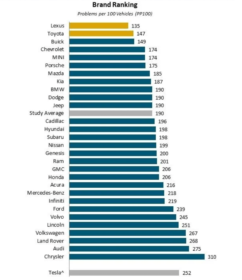
In systematic trading, statistics are our bread and butter. But not only in finance are statistical estimates ubiquitous; statistics are used to guide decision making in diverse fields, from medicine to insurance and politics. Some statistics, however, might not be that relevant to a single individual faced with making one single choice between different alternatives. Vehicle dependability studies, such as those conducted by J.D. Power (2024 Most Reliable Vehicles – U.S. Dependability Study), publish the average number of problems owners have experienced with their vehicle (reported as the number of problems per 100 vehicles) to rank car brands.
J.D. Power
2024 U.S. Vehicle Dependability Study℠
Rankings are based on numerical scores, and not necessarily on statistical significance.
At first glance, such a ranking appears to contain very useful information for an individual looking to buy a car. If reliability were the sole factor, people would navigate towards models on the top of the list, as these cars on average seem to have fewer problems. The challenge, however, is that most people will buy only one car- not thousands (unlike car warranty policy underwriters who consider large samples), and therefore the average number of problems a car might experience is not as relevant, or at least should be interpreted differently.
To help us make sense of those averages, we can look at the act of buying one car and not another as a random “experiment”: i.e. a random draw of car A (from brand A) versus a random draw of car B (from brand B) and ask ourselves some questions:
- “What is the probability that car A has fewer problems than car B?”
- “What is the probability that car A has the same number of problems as car B?”
- “What is the probability that car A has more problems than car B?”
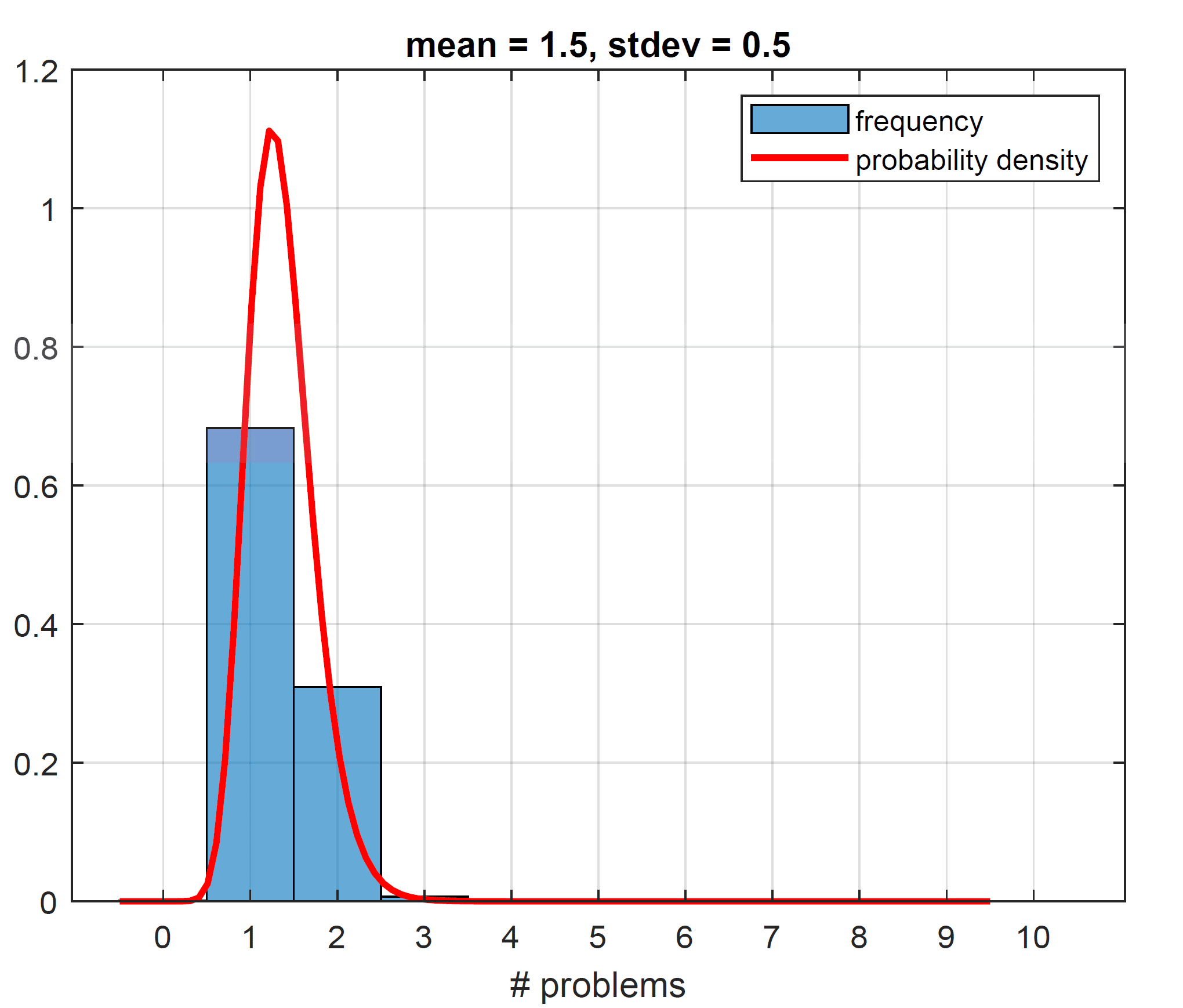
First, we need to assume a reasonable probability distribution to model the number of problems per car. A normal distribution, which is often our default choice, won’t work well here because it allows negative values. A lognormal distribution (where the natural logarithm of the random variable is normally distributed) is better suited here, as it models strictly non-negative variables. We will go one step further in finding a good model: the number of problems a car can have will always be measured in whole numbers, and to deal with these discrete outcomes, we will “transform” our continuous lognormal probability density function into discrete probabilities by binning values.
By varying parameters for the underlying lognormal distribution, we can design discrete distributions with means (and standard deviations) as needed. We want the means to reflect those observed in the J.D.Power ranking, ranging say from 1.35 problems per car (Lexus) to about 2.6 problems per car (Volkswagen or Land Rover), which is reasonable, because the action of calculating the sample mean is an “unbiased estimator” in statistical parlance. We also want the standard deviations to be realistic. To “choose” realistic standard deviations, we allude to “statistical fact”, “visual inspection” and some back-of-the-envelope heuristics.
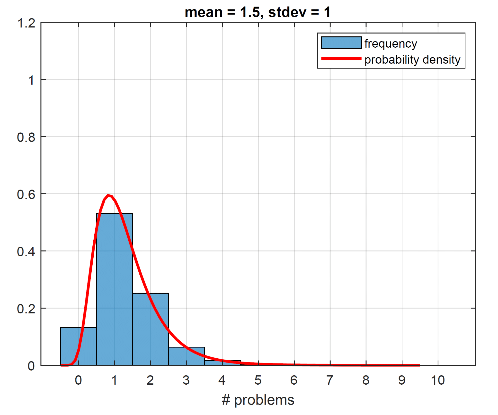
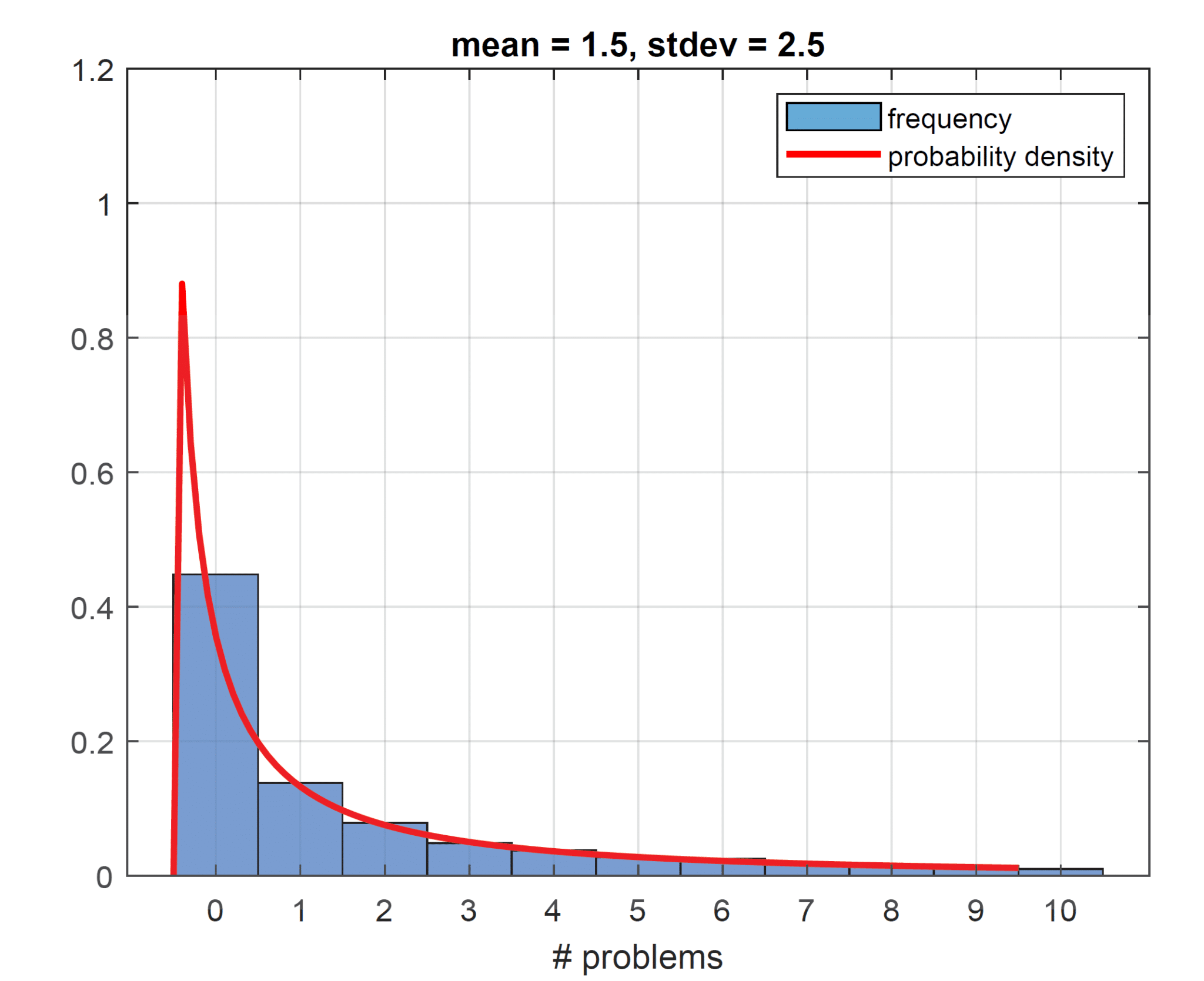
“Statistical fact” tells us that there must be some variability around how many problems each car has, purely because the averages are non-integers. If you buy a Toyota, and the ranking tells us that this brand has about 1.5 problems per car on average, it implies that some Toyotas must have two problems (or more). Placing a roughly equal probability on 1 or 2 problems (and no probability on zero problems) puts a floor on the permissible standard deviation of 0.5. So, at the very least, our standard deviation has to be 0.5. Generating our histogram (from the driving lognormal probability distribution, which we also plot for completeness) to result in a mean of 1.5 and a standard deviation of 0.5, we get the plot on the left below. Curiously the number of problems with the highest frequency ends up being 1 at a whopping 68%. The way the histogram looks is a result of the features of the lognormal distribution. When we pin down our mean, here at 1.5, and we postulate a low standard deviation, such as 0.5, we suppress the right tail of the lognormal and push more weight into the belly of the distribution (as the right tail heavily influences the standard deviation with no left tail to speak of here, since all values are strictly positive). This is why our lognormal density function looks more Gaussian for these parameters. Having the mode of the distribution (the point with the most frequent number of problems) sit at 1 seems unreasonable. We would expect most of the cars to have no problems and few cars to have many problems. Increasing the standard deviation to 1, we allow for a thicker right tail. This makes our histogram slightly more realistic (see the plot on the right below), though the mode is still at 1 with a frequency of 53%.
Bumping the standard deviation to a value of 2, the most frequent number of problems now equals 0, with a frequency of 40% (plot on the left below), so we could argue that our standard deviation should be at least 2. Increasing the standard deviation to 2.5 allows even more tail events, though they are still rare (plot on the right below). To maintain the mean of 1.5, the frequency of exactly no problem increases further to 45%.
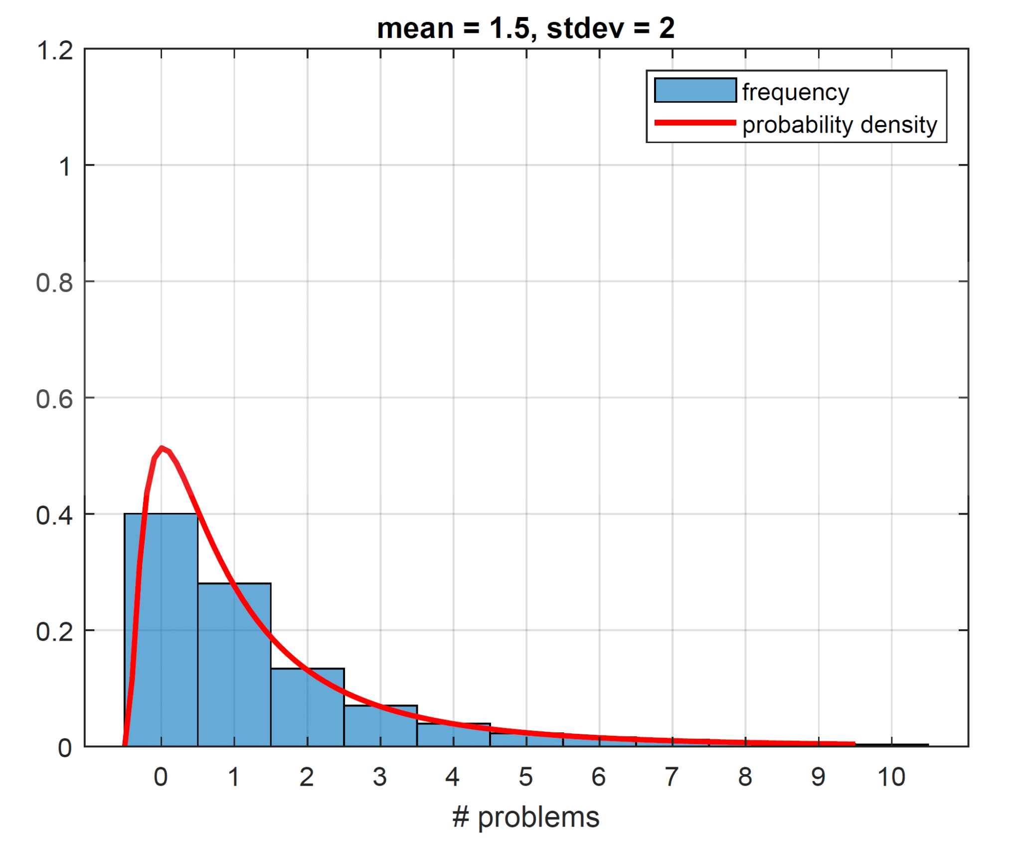
The plots shown suggest a standard deviation for the average number of problems a car has of about 2 to 3. We have one more way of supporting this estimate, using some heuristics.
J.D. Power only includes cars in their ranking for which they have a response size of at least 100 (see Syndicated Surveys FAQs | J.D. Power). We can estimate the number of responses per brand from the total sales figures for 2021 (about 15 million across all brands, found online) and the total number of survey responses provided by J.D. Power (30,595, see 2024 Most Reliable Vehicles – U.S. Dependability Study), by stipulating that the relative frequency of survey responses matches that of the sales. The top two most sold cars are Toyota and Ford, with 2,300,000 and 1,800,000 sales, respectively, while Mini and Jaguar had sales of 50,000 and 30,000, respectively. The smallest brand to be included is the Mini with an estimated number of samples of 100 exactly, while the largest brand to be excluded, Jaguar, is estimated at 60 samples.
The reason that the ranking excludes cars with a small response sample size is tied to statistical significance. The average number of problems per car brand reported in the survey is the sample mean. The bigger the sample, the more accurate this estimate becomes, with the sample mean approaching the true underlying mean. We can quantify the measurement error ε in the sample mean. In fact, it scales with the number of samples N (here the number of responses) and with the standard deviation around the average number of problems per car that we have been trying to estimate above. Let us now denote this standard deviation as Σ, and write down the expression for the measurement error:

If we have infinitely many samples, the measurement error is zero. If we only have one sample, the measurement error equals the standard deviation of car brand problems Σ.
To help us back up our estimate for Σ, we appeal to a statistical criterion of whether a car brand is included in the ranking or not. A reasonable such criterion is: Is its sample mean measurement error ε less than the cross-sectional standard deviation of sample means across all brands? We believe this is the minimum requirement to say that a brand belongs somewhere in the ranking with some statistical confidence. The latter cross-sectional standard deviation, if weighted by estimated sample size, is 0.35 problems. Cars that do not make it into the ranking, those with a sample size less than 100, are deemed to have an error ε too large to position them in the ranking. Using N = 100 and our cross-sectional standard deviation of 0.35 results in Σ = 3.5. This estimate of the standard deviation Σ falls towards (or just outside of) the top range of values we considered when plotting our histograms. A standard deviation between 2 and 3 is therefore what we settle on.
We have spent a lot of time trying to estimate a defensible range for Σ. Now we can finally return to the real question, or rather questions, asked at the beginning of this post. To answer them, we first determine the probability of a car (with a given mean and standard deviation) having a number of problems equal to n. We tabulate such values below for a range of means (reflecting the numbers reported by J.D. Power) and standard deviations (in line with our estimates). Note that these are effectively the frequencies we plotted in our histograms. Also note that we have specified the model in such a way that an increase in mean also implies a small increase in standard deviation, effectively saying that car brands that are better at lowering the average number of problems are also better at controlling the standard deviation.i
The table below is then read as follows: A car with an average number of problems equal to 1.35, such as a Lexus, has a 5% probability of having exactly three problems. A car with an average number of problems equal to 2.35, close to a Ford, has a 17% chance of having exactly one problem.
| Mean Standard deviation | 1.35 2.12 | 1.60 2.28 | 1.85 2.42 | 2.10 2.54 | 2.35 2.65 | 2.60 2.73 |
|---|---|---|---|---|---|---|
| n | P(n) | P(n) | P(n) | P(n) | P(n) | P(n) |
| 0 | 0.49 | 0.43 | 0.37 | 0.31 | 0.26 | 0.22 |
| 1 | 0.18 | 0.18 | 0.18 | 0.18 | 0.17 | 0.16 |
| 2 | 0.09 | 0.10 | 0.10 | 0.11 | 0.11 | 0.11 |
| 3 | 0.05 | 0.06 | 0.07 | 0.07 | 0.07 | 0.08 |
| 4 | 0.04 | 0.04 | 0.05 | 0.05 | 0.06 | 0.06 |
| 5 | 0.03 | 0.03 | 0.04 | 0.04 | 0.04 | 0.05 |
| 6 | 0.02 | 0.02 | 0.03 | 0.03 | 0.03 | 0.04 |
| 7 | 0.01 | 0.02 | 0.02 | 0.02 | 0.03 | 0.03 |
| 8 | 0.01 | 0.01 | 0.02 | 0.02 | 0.02 | 0.03 |
| 9 | 0.01 | 0.01 | 0.01 | 0.02 | 0.02 | 0.02 |
| 10 | 0.01 | 0.01 | 0.01 | 0.01 | 0.02 | 0.02 |
This table is now our workhorse. By multiplying and summing probabilitiesii, we can generate the more interesting table below, which lists for cars A (specified in each row) and B (specified in each column) the probability that car A has fewer/the same/more problems than car B. If we wanted to compare Lexus and Land Rover, for example, the best match would be to go to row 1.35, column 2.6, and read off 55%, 21% and 24%. We have a close to coin toss chance of Lexus having fewer problems than Land Rover, which is much less significant than the ranking would suggest.
| P(number of problems for car A) <|=|> P(number of problems for car B) | ||||||
|---|---|---|---|---|---|---|
| A/B | 1.35 | 1.60 | 1.85 | 2.10 | 2.35 | 2.60 |
| 1.35 | 34% | 32% | 34% | 38% | 30% | 32% | 43% | 27% | 30% | 47% | 25% | 28% | 51% | 23% | 26% | 55% | 21% | 24% |
| 1.60 | 32% | 30% | 38% | 36% | 28% | 36% | 41% | 25% | 34% | 45% | 23% | 32% | 49% | 21% | 30% | 52% | 20% | 28% |
| 1.85 | 30% | 27% | 43% | 34% | 25% | 41% | 38% | 23% | 38% | 42% | 22% | 36% | 46% | 20% | 34% | 50% | 19% | 32% |
| 2.10 | 28% | 25% | 47% | 32% | 23% | 45% | 36% | 22% | 42% | 40% | 20% | 40% | 44% | 19% | 37% | 50% | 19% | 32% |
| 2.35 | 26% | 23% | 51% | 30% | 21% | 49% | 34% | 20% | 46% | 37% | 19% | 44% | 41% | 18% | 41% | 45% | 17% | 39% |
| 2.60 | 24% | 21% | 55% | 28% | 20% | 52% | 32% | 19% | 50% | 35% | 18% | 47% | 39% | 17% | 45% | 42% | 16% | 42% |
Without being too serious, it looks like it is ok to buy a car based on more than its ranking, given that for an individual vehicle, most reliability comparisons won’t drastically favor one car over another.
On a more serious note, if thinking about investing, we can draw some analogy to performance metrics. When thinking about long-term performance, statistics matter. We care about averages over many samples, such as IRs.
If, however, we only place one bet (or buy one car), other factors come into play. We are actually reminded here of the “you-only-live-once” trades like GameStop, where investors might behave “as if they are buying one single car”. Maybe our thinking process offers a rational explanation for this apparently extreme behavior.
iHere we mainly make this choice to reduce the degrees of freedom of our underlying lognormal problem. We appeal to one single family of continuous lognormal distributions where for our lognormal random variable X we have X=eμ+σZ where Z is normal. We employ different μ, the expected value or mean of ln(X) and, for simplicity, the same σ, which is its standard deviation. The mean and standard deviation of X itself are both functions of μ and σ, so even with keeping σ constant an increase in μ will increase the standard deviation of X.
iiWe make use of two identities:
– For independent events, P(A and B) = P(A) P(B)
– P(A < n) = P(A=0) + P(A=1) + P(A=2) + … + P(A = n-1)
DISCLOSURE
This presentation includes statements that may constitute forward-looking statements. These statements may be identified by words such as “expects,” “looks forward to,” “anticipates,” “intends,” “plans,” “believes,” “seeks,” “estimates,” “will,” “project” or words of similar meaning. In addition, our representatives may from time to time make oral forward-looking statements. Such statements are based on the current expectations and certain assumptions of Graham Capital Management’s (“GCM”) management, and are, therefore, subject to certain risks and uncertainties. A variety of factors, many of which are beyond GCM’s control, affect the operations, performance, business strategy and results of the accounts that it manages and could cause the actual results, performance or achievements of such accounts to be materially different from any future results, performance or achievements that may be expressed or implied by such forward-looking statements or anticipated on the basis of historical trends.
This document is not a private offering memorandum and does not constitute an offer to sell, nor is it a solicitation of an offer to buy, any security. The views expressed herein are exclusively those of the authors and do not necessarily represent the views of Graham Capital Management. The information contained herein is not intended to provide accounting, legal, or tax advice and should not be relied on for investment decision making.
Tables, charts and commentary contained in this document have been prepared on a best efforts basis by Graham using sources it believes to be reliable although it does not guarantee the accuracy of the information on account of possible errors or omissions in the constituent data or calculations. No part of this document may be divulged to any other person, distributed, resold and/or reproduced without the prior written permission of GCM.
